Root[{{f1,…,fn},{c1,…,cn}},j]
represents the j![]() coordinate of the exact root of the system of equations {f1[x1,…,xn]0,…,fn[x1,…,xn]0} near {x1,…,xn}={c1,…,cn}.
coordinate of the exact root of the system of equations {f1[x1,…,xn]0,…,fn[x1,…,xn]0} near {x1,…,xn}={c1,…,cn}.
Root[f,k]
represents the exact k![]() root of the polynomial equation f[x]0.
root of the polynomial equation f[x]0.
Root[{f1,f2,…},{k1,k2,…}]
represents the last coordinate of the exact vector {a1,a2,…} such that ai is the ki![]() root of the polynomial equation fi[a1,…,ai-1,x]0.
root of the polynomial equation fi[a1,…,ai-1,x]0.


Root
Root[{f,c}]
represents the exact root of the general equation f[x]0 near x=c.
Root[{{f1,…,fn},{c1,…,cn}},j]
represents the j![]() coordinate of the exact root of the system of equations {f1[x1,…,xn]0,…,fn[x1,…,xn]0} near {x1,…,xn}={c1,…,cn}.
coordinate of the exact root of the system of equations {f1[x1,…,xn]0,…,fn[x1,…,xn]0} near {x1,…,xn}={c1,…,cn}.
Root[f,k]
represents the exact k![]() root of the polynomial equation f[x]0.
root of the polynomial equation f[x]0.
Root[{f1,f2,…},{k1,k2,…}]
represents the last coordinate of the exact vector {a1,a2,…} such that ai is the ki![]() root of the polynomial equation fi[a1,…,ai-1,x]0.
root of the polynomial equation fi[a1,…,ai-1,x]0.
Details and Options
- Root is also known as an algebraic number when f is polynomial with integer coefficients or a transcendental number when there is no such polynomial f possible.
- Root is typically used to represent an exact number and is automatically generated by a variety of algebra, calculus, optimization and geometry functions.
- Root represents an exact number as a solution to an equation f[x]0 with additional information specifying which of the roots is intended.
- Root numbers can be used like any other numbers, both in exact and approximate computations.
- Root numbers are formatted as
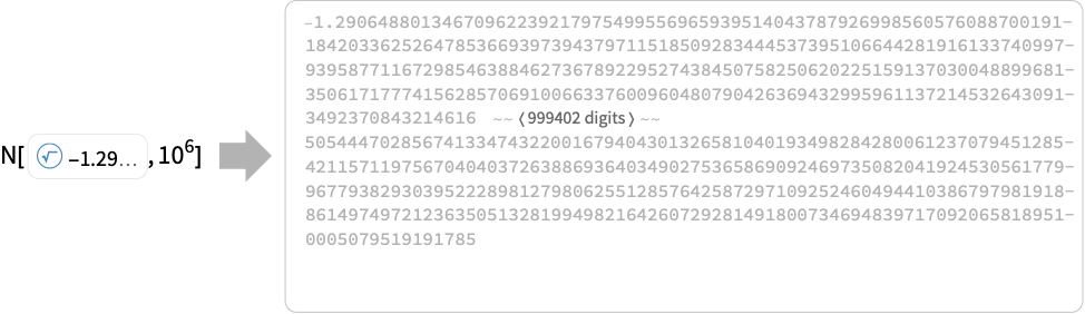
 where approx is a numerical approximation. An approximation to precision p can be computed using N[
 ,p].
,p]. - For most uses, Root objects are automatically generated and can be directly used. For advanced uses, when your code is going to directly generate Root objects, a deeper understanding of the different representations is necessary.
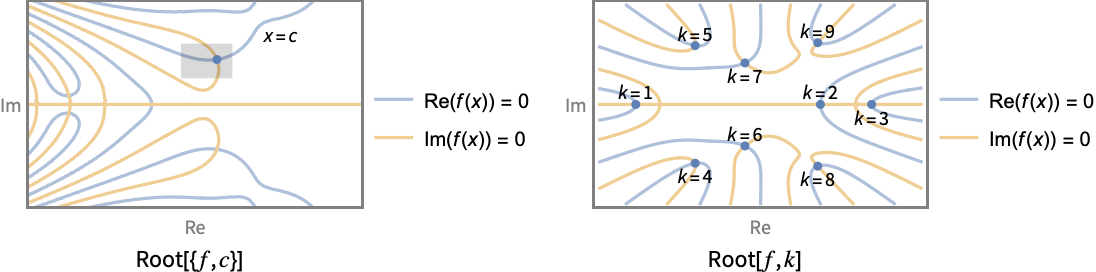
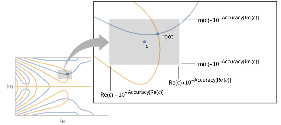
- There are two distinct mechanisms used to specify which root of an equation is represented, the neighborhood representation Root[{f,c}] and the indexing representation Root[f,k].
- The root neighborhood representation Root[{f,c}] specifies the equation f[x]0 as well as the neighborhood rectangle centered at c and width
 and height
  .
. - The root neighborhood representation for systems Root[{{f1,…,fn},{c1,…,cn}},j] similarly specifies a system of equations {f1[x1,…,xn]0,…,fn[x1,…,xn]0} and a neighborhood given by the product of rectangles from ci for the different coordinates.
- The root neighborhood representation Root[{f,c,m}] specifies that f[x]0 has a root of multiplicity m in the neighborhood given by c. However, it may be a cluster of closely spaced roots and by refining the neighborhood c, i.e. higher precision root approximation, they may separate. »
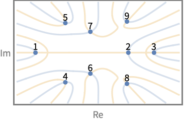
- The root indexing representation Root[f,k] applies to polynomial functions f only. The indexing of roots takes the real roots first, in increasing order. For polynomials with rational coefficients, the complex conjugate pairs of roots have consecutive indices.
- The root indexing representation for systems Root[{f1,f2,…,fk},{k1,k2,…,kn}] applies to triangular systems of polynomial equations only. Given equations f1[x1]0, f2[x1,x2]0, …, fn[x1,x2,…,xn]0, we recursively define r1 as the k1
") root of f1[x1]0, r2 as the k2
root of f1[x1]0, r2 as the k2") root of f2[r1,x2]0 and finally rn as the kn
root of f2[r1,x2]0 and finally rn as the kn") root of fn[r1,…,rn-1,xn]0. The represented root is rn.
root of fn[r1,…,rn-1,xn]0. The represented root is rn.
Examples
open all close allBasic Examples (4)
Solve[x ^ 5 + 2x + 1 == 0, x]N[%]Real solutions to an exp-log equation:
Reduce[E ^ x - 5x + Log[2 x] + 1 == 0, x, Reals]Real solution to a system of equations:
Solve[x ^ 5 - x == 2 && y ^ 5 - x ^ 2 y == 3, {x, y}, Reals]A solution instance to a system of transcendental equations:
FindInstance[Sin[x E ^ y] - x == 1 && Gamma[x - Cos[y]] == Erf[x + y], {x, y}]Scope (22)
Basic Uses (5)
Some exact values are generated automatically:
Root[# ^ 2 - 3# - 1&, 2]Root[# ^ 5 - 3#&, 2]Root[{#1 ^ 2 - 3&, #2 ^ 2 - #1 - 5&}, {1, 2}]Root[{Sin[#]&, 3.1415926535897932385}]N[Root[# ^ 7 - 3# + 1&, 1], 100]N[Root[{#1 ^ 7 - 3#1 + 1&, #2 ^ 7 - #1 ^ 2#2 - 5&, #3 ^ 7 - #2 ^ 2#3 - #1 + 1&}, {1, 2, 3}], 100]N[Root[{1 + E ^ #1 + Log[2#1] - 5#1&, 2.071312961691322349521}], 100]Root[# ^ 6 - 11# + 1&, 1] < Sqrt[2]Convert radicals to a Root object:
RootReduce[Sqrt[2] + Sqrt[3]]Convert a Root object to radicals:
ToRadicals[%]Disable the elided formatting of Root:
SetSystemOptions["TypesetOptions" -> {"NumericalApproximationForms" -> False}];Reduce[x ^ 3 - 2x + 7 == 0, x]Re-enable the elided formatting:
SetSystemOptions["TypesetOptions" -> {"NumericalApproximationForms" -> True}];Reduce[x ^ 3 - 2x + 7 == 0, x]Roots of Univariate Functions (4)
Real roots of an exp-log function:
Reduce[E ^ (2E ^ x) - Log[x ^ 2 + 1] - 20x == 11, x, Reals]The Root representation involves a univariate function and an approximation that isolates the root:
r = %[[2, 2]]List@@rThe Root object is an exact numeric expression:
Log[r] < 1 / 2N[r, 50]Roots of an analytic function in a bounded region:
Reduce[2Sin[Exp[x]] - Cos[Pi x] == 1 / 3 && Abs[x] < 1, x]Reduce[Cos[3x] - 6x Cos[2x] + (12x ^ 2 + 3)Cos[x] - 4x ^ 3 - 6x == 0 && Abs[x] < 1, x]List@@%[[2]]This representation is used for roots of polynomials of degrees that exceed $MaxRootDegree:
Reduce[x ^ 1234567 + 5 x + 1 == 0, x, Reals]r = %[[2]]List@@rThe approximation used to represent the root is equal to ![]() , but the root is not:
, but the root is not:
Block[{$MaxExtraPrecision = Infinity}, N[r + 1 / 5, 20]]Roots of Multivariate Systems (1)
Find a solution instance to a system of transcendental equations:
FindInstance[Exp[x - y] == 2 + Sin[x y] && Tan[x / y] == 5x - y, {x, y}]The roots are exact numeric expressions:
r = x /. %[[1]]N[r, 50]The Root representation involves a multivariate system and an approximation that isolates the root:
List@@rRoots of Univariate Polynomials (10)
Roots of a univariate polynomial with rational coefficients are algebraic numbers:
SolveValues[x ^ 5 - 3x + 7 == 0, x]Element[%, Algebraics]The polynomials are automatically reduced:
r = Root[3# ^ 7 - 3&, 3]A minimal polynomial is always irreducible and primitive:
First[%]Use MinimalPolynomial to extract the minimal polynomial:
MinimalPolynomial[%%, x]A Root object representing an algebraic number has three arguments:
r = Root[# ^ 7 - 4# ^ 3 + 9&, 5]The third argument is 0 (default value) or 1 and indicates the root isolation method to be used:
List@@rThe root isolation method used may affect the ordering of non-real roots:
Root[# ^ 7 - 4# ^ 3 + 9&, 5, 1]% ≠ rRoots of polynomials of degree at 1 and 2 simplify automatically:
Root[2# + 3&, 1]Root[7 # ^ 2 + 8 # + 9&, 2]An algebraic combination of algebraic numbers is an algebraic number:
Sqrt[Root[# ^ 3 - 2# - 7&, 1]] + 2Root[# ^ 4 - 5# - 9&, 3] ^ 2Use RootReduce to represent the result as a single Root object:
RootReduce[%]The canonicalization is not done automatically since minimal polynomials can grow rapidly:
MinimalPolynomial[%, x]Complex components of algebraic numbers:
Re[Root[# ^ 6 - # + 1&, 1]]//RootReduceAbs[Root[# ^ 6 - # + 1&, 1]]//RootReduceRoot of a polynomial with exact numeric coefficients is an exact numeric object:
Root[# ^ 3 + Pi # + I ^ E&, 1]Abs[%] < 2N[%%, 50]Roots of a polynomial with coefficients involving symbolic parameters:
SolveValues[x ^ 5 - 2a x + a ^ 2 == 1, x]Plot[%, {a, -5, 5}, WorkingPrecision -> 20]Find the series with respect to the parameter:
Series[First[%%], {a, 0, 10}]Find Puiseux series of a root at a branch point:
Series[Root[Function[x, x ^ 3 - x ^ 2 - x + a], 2], {a, 1, 2}]Roots of a quadratic with symbolic coefficients:
{Root[a # ^ 2 + b # + c&, 1], Root[a # ^ 2 + b # + c&, 2]}When a, b, c and the roots are real, the roots are always ordered by their values:
% /. {{a -> 1, b -> -3, c -> 2}, {a -> -1, b -> 3, c -> -2}}The "standard" formulas for the roots of a quadratic do not guarantee the ordering of roots:
SolveValues[a x ^ 2 + b x + c == 0, x]% /. {{a -> 1, b -> -3, c -> 2}, {a -> -1, b -> 3, c -> -2}}Roots of Triangular Polynomial Systems (2)
Real root of a triangular system of equations:
FindInstance[x ^ 5 - x == 2 && y ^ 5 - x ^ 2 y == 3 && z ^ 5 - x ^ 3 y ^ 2 z == 5, {x, y, z}, Reals]The Root representation involves a triangular polynomial system and root indices:
r = z /. %[[1]]List@@rThe Root object is an exact numeric expression:
r == 163 / 100N[r, 50]Roots of systems of polynomials with rational coefficients have algebraic number coordinates:
Element[r, Algebraics]The degree of the minimal polynomial is generally the product of degrees of the system polynomials:
MinimalPolynomial[r, x]This representation is used for roots of polynomials with algebraic number coefficients:
r = Root[# ^ 5 + Sqrt[2]# + 1&, 1]List@@rConvert the root to the canonical algebraic number representation:
s = RootReduce[r]List@@sOptions (1)
ExactRootIsolation (1)
Root[f,k] by default isolates the complex roots of a polynomial using validated numerical methods. Setting ExactRootIsolationTrue will make Root use symbolic methods that are usually much slower.
The setting of ExactRootIsolation is reflected in the third argument of a Root object:
a = Root[# ^ 40 - 15# ^ 17 - 21# ^ 3 + 11&, 20, ExactRootIsolation -> False];
b = Root[# ^ 40 - 15# ^ 17 - 21# ^ 3 + 11&, 20, ExactRootIsolation -> True];{a, b}//InputFormRoot isolation is performed the first time the numerical value of the root is needed:
N[a, 20]//TimingThe symbolic complex root isolation method is usually slower than the validated numeric one:
N[b, 20]//TimingThe root isolation method may affect the ordering of nonreal roots:
N[{Root[# ^ 20 - 15# ^ 17 - 21# ^ 3 + 11&, 20, ExactRootIsolation -> True], Root[# ^ 20 - 15# ^ 17 - 21# ^ 3 + 11&, 20, ExactRootIsolation -> False]}, 20]Applications (19)
Solve polynomial equations of any degree in closed form in terms of Root:
First[Solve[(x + 1) ^ 20 + x - 2 == 0, x]]Solve the characteristic equation of a Hilbert matrix:
CharacteristicPolynomial[Table[1 / (i + j + 1), {i, 5}, {j, 5}], λ]Solve[% == 0, λ]//LastUsing Eigenvalues:
Eigenvalues[Table[1 / (i + j + 1), {i, 5}, {j, 5}]]//FirstFind the minimum of a parameterized polynomial:
Minimize[x ^ 4 + 3 x ^ 3 + a x - 1, x]Solve a constant coefficient differential equation of any degree:
DSolve[D[y[t], {t, 5}] + 11 D[y[t], {t, 1}] + y[t] == 0, y[t], t]Solve a constant coefficient difference equation of any degree:
RSolve[y[k + 5] + 11 y[k + 1] + y[k] == 0, y[k], k]Find a solution of a triangular system of equations:
FindInstance[x ^ 3 - 3x + 1 == 0 && y ^ 3 - x y + 2 == 0 && z ^ 3 - x y z + 3 == 0, {x, y, z}]Represent the solution in the Root[f,k] form:
RootReduce[%]Here, the Root[f,k] representation would involve a polynomial of degree 1000000:
FindInstance[x ^ 100 - 3x + 1 == 0 && y ^ 100 - x y + 2 == 0 && z ^ 100 - x y z + 3 == 0, {x, y, z}]Compute an approximate value of the solution:
N[%, 20]UnitStep[x ^ 6 + 5x - 1]PiecewiseExpand[%]Solve univariate exp-log equations and inequalities over the reals:
Reduce[E ^ x / x ^ 3 - (x + 1)Log[x] - Log[Log[x]] == 1, x, Reals]Reduce[x Log[x] - E ^ x > -2, x, Reals]Solve univariate elementary function equations over bounded intervals and regions:
Reduce[Sin[Cos[x]] - 4x ^ 2 + E ^ x == 1 && -1 < x < 1, x]Reduce[(x + 1) ^ Sin[x] == Cos[x ^ 2 - Tan[x]] + I / 2 && 0 ≤ Re[x] ≤ 1 && 0 ≤ Im[x] ≤ 1, x]Solve univariate analytic equations over bounded intervals and regions:
Reduce[Cos[x] - BesselJ[5, x] == 1 / 2 && 0 ≤ x ≤ 10, x]Reduce[Gamma[x] - Log[x] == 1 && Abs[x - 2] < 3 / 2, x]Find real roots of high-degree sparse polynomials and algebraic functions:
Reduce[x ^ 1000001 - 5x ^ 2 + 1 == 0, x, Reals]Reduce[Sqrt[x] - 3 x ^ (1 / 300000) + 5x ^ 2 == 0, x, Reals]Solve univariate transcendental optimization problems:
Minimize[{E ^ (x E ^ x) + x ^ Log[x], x > 0}, x]Maximize[{Sin[Cos[x]] - Exp[(x - 1) ^ 2], 0 < x < 2}, x]Integrate a piecewise function with an exp-log inequality condition:
Integrate[x Boole[E ^ x - x ^ x > 2], {x, 0, Infinity}]Evaluate the hard hexagon entropy constant:
N[Root[-32751691810479015985152 + 97143135277377575190528# ^ 4 -
	73347491183630103871488 # ^ 6 - 71220809441400405884928 # ^ 8 +
	107155448150443388043264# ^ 10 - 72405670285649161617408 # ^ 12 +
    2958015038376958230528# ^ 14 + 7449488310131083100160# ^ 16 +
	797726698866658379776# ^ 18 + 2505062311720673792#1 ^ 20 +
2013290651222784# ^ 22 + 25937424601# ^ 24&, 2] , 20]Reduce[x - Sin[x] / 2 == 1 && 0 <= x <= 2, x]Compute the Laplace limit constant:
Reduce[y E ^ Sqrt[1 + y ^ 2] / (1 + Sqrt[1 + y ^ 2]) == 1, y, Reals]N[%[[2]], 100]Plot a root as a function of a parameter:
Plot[Re[Root[# ^ 5 + a # + 1&, 1]], {a, -5, 5}]Solve a convex optimization problem:
Minimize[{v.{-1, 1}, {{1, 0}, {0, 1}, {-1, -2}}.vUnderscript[, "ExponentialCone"]{0, 0, -2}}, v]Find a solution instance of a system of transcendental equations and inequalities:
FindInstance[Exp[x + y] + Sin[z] == x z && Log[z ^ 2 - x] == Erf[x - 2y] + 1 && Tan[x ^ y] < z - 2, {x, y, z}, Reals]Properties & Relations (11)
Root objects represent exact numbers:
Root[# ^ 5 - 3# + 4&, 1]Compute approximations to arbitrary precision:
N[%, 50]SolveValues[Sin[x] - Log[x] / x == 0 && 0 < x < 10, x]N[Last[%], 50]Use MinimalPolynomial to find minimal polynomials of algebraic numbers:
Root[# ^ 5 + # + 1&, 1]MinimalPolynomial[%, x]Root[{#1 ^ 3 + 7#1 + 11&, #2 ^ 5 - 3#1 #2 + 5#1 ^ 2 + 1&}, {2, 3}]MinimalPolynomial[%, x]Use ToRadicals to attempt to convert a Root object to an arithmetic combination of radicals:
root = Root[# ^ 3 + # + 11&, 1]All roots of polynomials of degree not exceeding 4 are representable in radicals:
ToRadicals[root]Use RootReduce to canonicalize algebraic numbers, including from operations:
Root[# ^ 5 + # + 1&, 1] ^ (1 / 3)RootReduce[%]Root[# ^ 5 + # + 1&, 1] - Root[# ^ 6 - # + 1&, 1]RootReduce[%]Root[{#1 ^ 3 - 3#1 + 1&, #2 ^ 3 - #1 ^ 2#2 - 5&, #3 ^ 3 - #2 ^ 2#3 - #1 + 1&}, {1, 2, 3}]RootReduce[%]Use AlgebraicNumber for computations within a fixed simple extension of the rationals:
a = AlgebraicNumber[Root[# ^ 5 - 2# + 7&, 1], {0, 1}]Rational operations on AlgebraicNumber objects produce AlgebraicNumber objects:
(5a ^ 3 + 7a + 9) / (15a ^ 4 - 11a + 3)Use ToNumberField to express given algebraic numbers as elements of the same simple extension:
{a, b, c} = {Root[# ^ 3 + 3# - 5&, 1], Root[# ^ 5 + 2# + 7&, 1], Sqrt[5]}{aa, bb, cc} = ToNumberField[{a, b, c}]RootReduce[{a, b, c} - {aa, bb, cc}]Perform computations within the common simple extension or rationals:
(aa ^ 2 - bb cc) / (bb ^ 3 - 3aa + cc ^ 2)RootSum represents the sum of values of a function over roots of a polynomial:
RootSum[# ^ 5 - 3# + 5&, Sin[#]&]Use Normal to represent the sum using explicit roots:
Normal[%]For rational functions, the sum can be computed without finding the roots:
RootSum[# ^ 5 - 3# + 5&, (# ^ 3 - 5# + 12) / (2# ^ 7 - 3# ^ 4 + 6# - 9)&]Simplify combinations of Root objects:
Product[Root[2# ^ 5 + 4# + 1&, i], {i, 5}]FullSimplify[%]Solve an equation for a parameter in a Root object:
Solve[Root[# ^ 5 + a # + 2a ^ 2&, 1] == -3, a]Use ImplicitD to compute derivatives of implicit solutions of equations:
r = Root[# ^ 5 - x # + 1&, 1]ImplicitD[r[[1]][y] == 0, y, x]Compare with the result obtained by computing the derivative of ![]() directly:
directly:
(% /. y -> r) == D[r, x]Compute series expansions of implicit solutions to equations:
Series[Root[# ^ 5 + a # + 1&, 1], {a, 0, 10}]% ^ 5 + a % + 1Use AsymptoticSolve to find series expansions of all roots:
AsymptoticSolve[x ^ 5 + a x + 1 == 0, x, {a, 0, 5}]Use RootApproximant to generate Root objects that approximate given numbers:
RootApproximant[Sqrt[2.] + Sqrt[3.]]RootApproximant[N[Pi, 10]]Possible Issues (5)
Series at branch points may not be valid in all directions:
Series[Root[Function[x, x ^ 3 - x ^ 2 - x + a], 2], {a, 1, 2}]Canonicalization is only possible for parameter‐free roots:
RootReduce[Sqrt[Root[# ^ 5 + # + a&, 1] ]]Parameterized roots can have complicated branch cuts in the complex parameter plane:
ContourPlot[With[{z = x + I y}, Arg[Root[# ^ 5 + (z ^ 2 - 1)# ^ 3 - 1 / z # ^ 2 + (z - I) ^ 3 - z&, 4] ]], {x, -2, 2}, {y, -2, 2}, Exclusions -> None]A non-polynomial Root object may represent a cluster of distinct roots:
f = Evaluate[Expand[(Sin[#] - 1 - I 10 ^ -100)(Sin[#] - 1 + I 10 ^ -100)]]&;cluster = Root[{f, N[Pi / 2, 20]}]Numerical computation with a higher precision yields an approximation of one of the roots:
N[cluster, 100]
The choice of root stays the same for subsequent computations:
N[cluster, 200]A larger setting for $MaxExtraPrecision can be needed for roots with noninteger coefficients:
Root[Function[x, Evaluate[(Rationalize[Pi, 10 ^ -200] - Pi)x ^ 3 + 2 x - 1]], 1]
Block[{$MaxExtraPrecision = 200}, Root[Function[x, Evaluate[(Rationalize[Pi, 10 ^ -200] - Pi)x ^ 3 + 2 x - 1]], 1]]Related Links
Text
Wolfram Research (1996), Root, Wolfram Language function, https://reference.wolfram.com/language/ref/Root.html (updated 2021).
CMS
Wolfram Language. 1996. "Root." Wolfram Language & System Documentation Center. Wolfram Research. Last Modified 2021. https://reference.wolfram.com/language/ref/Root.html.
APA
Wolfram Language. (1996). Root. Wolfram Language & System Documentation Center. Retrieved from https://reference.wolfram.com/language/ref/Root.html