 个坐标.
 次方根.


Root
 个坐标.
 次方根.
更多信息和选项
- 当 f 是系数为整数的多项式时,Root 也称为代数数,当这样的多项式不存在时,称为超越数.
- Root 通常用于表示一个精确的数字,由各种代数、微积分、优化和几何函数自动生成.
- Root 表示一个精确数,作为方程 f[x]0 的解,附加信息指定了哪个根是预期的.
- Root 数可以像任何其他数值一样用于精确和近似计算.
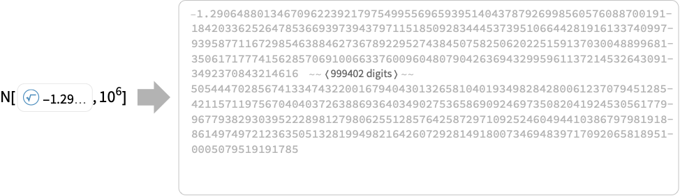
- Root 数的格式为
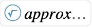 ,其中 approx 是一个数值近似. 精度为 p 的近似可以使用 N[
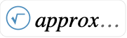 ,p] 计算.
- 对于大多数用途,Root 对象是自动生成的,可以直接使用. 对于高级用途,当您的代码要直接生成 Root 对象时,需要对不同的表示形式有更深入地了解.
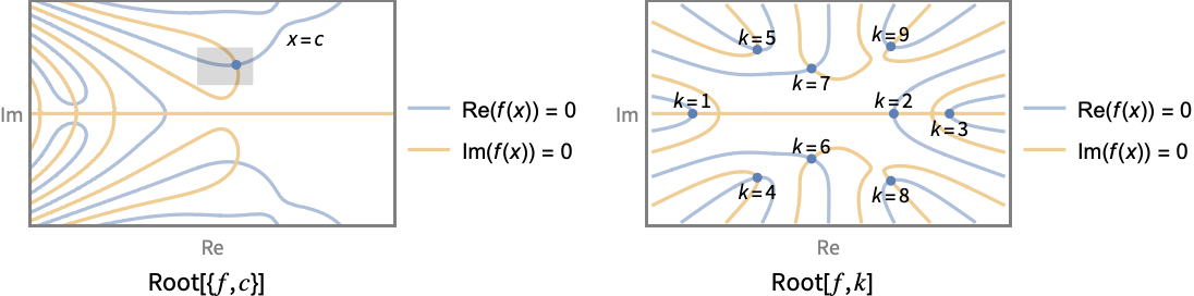
- 有两种不同的机制用于指定表示方程的哪个根,邻域表示 Root[{f,c}] 和索引表示 Root[f,k].
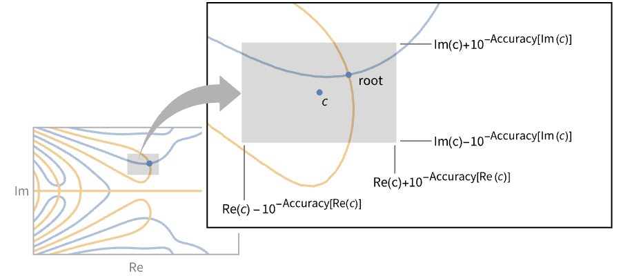
- 根邻域表示 Root[{f,c}] 指定方程 f[x]0,以及以 c 为中心,宽度为
 ,高度为
 的邻域矩形.
- 系统 Root[{{f1,…,fn},{c1,…,cn}},j] 的根邻域表示类似地指定一个方程组 {f1[x1,…,xn]0,…,fn[x1,…,xn]0} 和由来自 ci 的不同坐标的矩形乘积给出的邻域.
- 根邻域表示 Root[{f,c,m}] 指定 f[x]0 在由 c 给定的邻域中具有重数为 m 的根. 但这可能是一组间隔紧密的根,通过细化邻域 c,即更高精度的根近似,可能会将它们分开. »
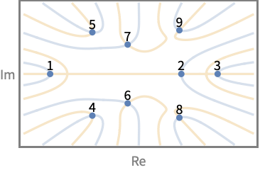
- 根索引表示 Root[f,k] 仅适用于多项式函数 f. 根的索引首先取实根,按升序排列. 对于具有有理系数的多项式,根的复共轭对具有连续的索引.
- 系统 Root[{f1,f2,…,fk},{k1,k2,…,kn}] 的根索引表示仅适用于多项式方程的三角系统. 已知方程f1[x1]0,f2[x1,x2]0,…,fn[x1,x2,…,xn]0,我们递归地定义 r1 为 f1[x1]0 的 k1
 次方根,r2 为 f2[r1,x2]0 的 k2
 次方根,……,rn 为 fn[r1,…,rn-1,xn]0 的 kn 次方根. 表示的根是 rn.
范例
打开所有单元 关闭所有单元基本范例 (4)
Solve[x ^ 5 + 2x + 1 == 0, x]N[%]Reduce[E ^ x - 5x + Log[2 x] + 1 == 0, x, Reals]Solve[x ^ 5 - x == 2 && y ^ 5 - x ^ 2 y == 3, {x, y}, Reals]FindInstance[Sin[x E ^ y] - x == 1 && Gamma[x - Cos[y]] == Erf[x + y], {x, y}]范围 (22)
基本用法 (5)
Root[# ^ 2 - 3# - 1&, 2]Root[# ^ 5 - 3#&, 2]Root[{#1 ^ 2 - 3&, #2 ^ 2 - #1 - 5&}, {1, 2}]Root[{Sin[#]&, 3.1415926535897932385}]N[Root[# ^ 7 - 3# + 1&, 1], 100]N[Root[{#1 ^ 7 - 3#1 + 1&, #2 ^ 7 - #1 ^ 2#2 - 5&, #3 ^ 7 - #2 ^ 2#3 - #1 + 1&}, {1, 2, 3}], 100]N[Root[{1 + E ^ #1 + Log[2#1] - 5#1&, 2.071312961691322349521}], 100]Root[# ^ 6 - 11# + 1&, 1] < Sqrt[2]将根式转换为 Root 对象:
RootReduce[Sqrt[2] + Sqrt[3]]将 Root 对象转换为根式:
ToRadicals[%]禁用 Root 的省略格式:
SetSystemOptions["TypesetOptions" -> {"NumericalApproximationForms" -> False}];Reduce[x ^ 3 - 2x + 7 == 0, x]SetSystemOptions["TypesetOptions" -> {"NumericalApproximationForms" -> True}];Reduce[x ^ 3 - 2x + 7 == 0, x]单变量函数的根 (4)
Reduce[E ^ (2E ^ x) - Log[x ^ 2 + 1] - 20x == 11, x, Reals]Root 表示涉及一个单变量函数和一个隔离根的近似值:
r = %[[2, 2]]List@@rRoot 对象是精确的数值表达式:
Log[r] < 1 / 2N[r, 50]Reduce[2Sin[Exp[x]] - Cos[Pi x] == 1 / 3 && Abs[x] < 1, x]Reduce[Cos[3x] - 6x Cos[2x] + (12x ^ 2 + 3)Cos[x] - 4x ^ 3 - 6x == 0 && Abs[x] < 1, x]List@@%[[2]]此表示用于次数超过 $MaxRootDegree 的多项式的根:
Reduce[x ^ 1234567 + 5 x + 1 == 0, x, Reals]r = %[[2]]List@@r
Block[{$MaxExtraPrecision = Infinity}, N[r + 1 / 5, 20]]多变量系统的根 (1)
FindInstance[Exp[x - y] == 2 + Sin[x y] && Tan[x / y] == 5x - y, {x, y}]r = x /. %[[1]]N[r, 50]Root 表示涉及一个多变量系统和一个隔离根的近似:
List@@r单变量多项式的根 (10)
SolveValues[x ^ 5 - 3x + 7 == 0, x]Element[%, Algebraics]r = Root[3# ^ 7 - 3&, 3]First[%]使用 MinimalPolynomial 提取最小多项式:
MinimalPolynomial[%%, x]代表代数数的 Root 对象具有三个参数:
r = Root[# ^ 7 - 4# ^ 3 + 9&, 5]List@@rRoot[# ^ 7 - 4# ^ 3 + 9&, 5, 1]% ≠ rRoot[2# + 3&, 1]Root[7 # ^ 2 + 8 # + 9&, 2]Sqrt[Root[# ^ 3 - 2# - 7&, 1]] + 2Root[# ^ 4 - 5# - 9&, 3] ^ 2使用 RootReduce 将结果表示为单个 Root 对象:
RootReduce[%]MinimalPolynomial[%, x]Re[Root[# ^ 6 - # + 1&, 1]]//RootReduceAbs[Root[# ^ 6 - # + 1&, 1]]//RootReduce具有精确数值系数的多项式的 Root 是一个精确数值对象:
Root[# ^ 3 + Pi # + I ^ E&, 1]Abs[%] < 2N[%%, 50]SolveValues[x ^ 5 - 2a x + a ^ 2 == 1, x]Plot[%, {a, -5, 5}, WorkingPrecision -> 20]Series[First[%%], {a, 0, 10}]Series[Root[Function[x, x ^ 3 - x ^ 2 - x + a], 2], {a, 1, 2}]
{Root[a # ^ 2 + b # + c&, 1], Root[a # ^ 2 + b # + c&, 2]}% /. {{a -> 1, b -> -3, c -> 2}, {a -> -1, b -> 3, c -> -2}}SolveValues[a x ^ 2 + b x + c == 0, x]% /. {{a -> 1, b -> -3, c -> 2}, {a -> -1, b -> 3, c -> -2}}三角多项式系统的根 (2)
FindInstance[x ^ 5 - x == 2 && y ^ 5 - x ^ 2 y == 3 && z ^ 5 - x ^ 3 y ^ 2 z == 5, {x, y, z}, Reals]Root 表示涉及三角多项式系统和根索引:
r = z /. %[[1]]List@@rRoot 对象是一个精确的数值表达式:
r == 163 / 100N[r, 50]Element[r, Algebraics]MinimalPolynomial[r, x]r = Root[# ^ 5 + Sqrt[2]# + 1&, 1]List@@rs = RootReduce[r]List@@s选项 (1)
ExactRootIsolation (1)
Root[f,k] 默认使用经过验证的数值方法隔离多项式的复根. 设置 ExactRootIsolationTrue 将使 Root 采用通常慢得多的符号方法.
ExactRootIsolation 的设置受到 Root 对象的第 3 个自变量的影响:
a = Root[# ^ 40 - 15# ^ 17 - 21# ^ 3 + 11&, 20, ExactRootIsolation -> False];
b = Root[# ^ 40 - 15# ^ 17 - 21# ^ 3 + 11&, 20, ExactRootIsolation -> True];{a, b}//InputFormN[a, 20]//TimingN[b, 20]//TimingN[{Root[# ^ 20 - 15# ^ 17 - 21# ^ 3 + 11&, 20, ExactRootIsolation -> True], Root[# ^ 20 - 15# ^ 17 - 21# ^ 3 + 11&, 20, ExactRootIsolation -> False]}, 20]应用 (19)
按照 Root 的封闭形式求解任意次数的多项式方程:
First[Solve[(x + 1) ^ 20 + x - 2 == 0, x]]CharacteristicPolynomial[Table[1 / (i + j + 1), {i, 5}, {j, 5}], λ]Solve[% == 0, λ]//Last用 Eigenvalues:
Eigenvalues[Table[1 / (i + j + 1), {i, 5}, {j, 5}]]//FirstMinimize[x ^ 4 + 3 x ^ 3 + a x - 1, x]DSolve[D[y[t], {t, 5}] + 11 D[y[t], {t, 1}] + y[t] == 0, y[t], t]RSolve[y[k + 5] + 11 y[k + 1] + y[k] == 0, y[k], k]FindInstance[x ^ 3 - 3x + 1 == 0 && y ^ 3 - x y + 2 == 0 && z ^ 3 - x y z + 3 == 0, {x, y, z}]以 Root[f,k] 格式表示解:
RootReduce[%]这里,Root[f,k] 表示法应该包含次数为 1000000 的多项式:
FindInstance[x ^ 100 - 3x + 1 == 0 && y ^ 100 - x y + 2 == 0 && z ^ 100 - x y z + 3 == 0, {x, y, z}]N[%, 20]UnitStep[x ^ 6 + 5x - 1]PiecewiseExpand[%]Reduce[E ^ x / x ^ 3 - (x + 1)Log[x] - Log[Log[x]] == 1, x, Reals]Reduce[x Log[x] - E ^ x > -2, x, Reals]Reduce[Sin[Cos[x]] - 4x ^ 2 + E ^ x == 1 && -1 < x < 1, x]Reduce[(x + 1) ^ Sin[x] == Cos[x ^ 2 - Tan[x]] + I / 2 && 0 ≤ Re[x] ≤ 1 && 0 ≤ Im[x] ≤ 1, x]Reduce[Cos[x] - BesselJ[5, x] == 1 / 2 && 0 ≤ x ≤ 10, x]
Reduce[Gamma[x] - Log[x] == 1 && Abs[x - 2] < 3 / 2, x]
Reduce[x ^ 1000001 - 5x ^ 2 + 1 == 0, x, Reals]Reduce[Sqrt[x] - 3 x ^ (1 / 300000) + 5x ^ 2 == 0, x, Reals]Minimize[{E ^ (x E ^ x) + x ^ Log[x], x > 0}, x]Maximize[{Sin[Cos[x]] - Exp[(x - 1) ^ 2], 0 < x < 2}, x]Integrate[x Boole[E ^ x - x ^ x > 2], {x, 0, Infinity}]N[Root[-32751691810479015985152 + 97143135277377575190528# ^ 4 -
73347491183630103871488 # ^ 6 - 71220809441400405884928 # ^ 8 +
107155448150443388043264# ^ 10 - 72405670285649161617408 # ^ 12 +
2958015038376958230528# ^ 14 + 7449488310131083100160# ^ 16 +
797726698866658379776# ^ 18 + 2505062311720673792#1 ^ 20 +
2013290651222784# ^ 22 + 25937424601# ^ 24&, 2] , 20]Reduce[x - Sin[x] / 2 == 1 && 0 <= x <= 2, x]Reduce[y E ^ Sqrt[1 + y ^ 2] / (1 + Sqrt[1 + y ^ 2]) == 1, y, Reals]N[%[[2]], 100]Plot[Re[Root[# ^ 5 + a # + 1&, 1]], {a, -5, 5}]Minimize[{v.{-1, 1}, {{1, 0}, {0, 1}, {-1, -2}}.vUnderscript[, "ExponentialCone"]{0, 0, -2}}, v]FindInstance[Exp[x + y] + Sin[z] == x z && Log[z ^ 2 - x] == Erf[x - 2y] + 1 && Tan[x ^ y] < z - 2, {x, y, z}, Reals]属性和关系 (11)
Root 对象代表精确的数:
Root[# ^ 5 - 3# + 4&, 1]N[%, 50]SolveValues[Sin[x] - Log[x] / x == 0 && 0 < x < 10, x]N[Last[%], 50]使用 MinimalPolynomial 求代数数的最小多项式:
Root[# ^ 5 + # + 1&, 1]MinimalPolynomial[%, x]Root[{#1 ^ 3 + 7#1 + 11&, #2 ^ 5 - 3#1 #2 + 5#1 ^ 2 + 1&}, {2, 3}]MinimalPolynomial[%, x]使用 ToRadicals 尝试将 Root 对象转换为根式的算术组合:
root = Root[# ^ 3 + # + 11&, 1]ToRadicals[root]用 RootReduce 规范化代数,包括来自操作:
Root[# ^ 5 + # + 1&, 1] ^ (1 / 3)RootReduce[%]Root[# ^ 5 + # + 1&, 1] - Root[# ^ 6 - # + 1&, 1]RootReduce[%]Root[{#1 ^ 3 - 3#1 + 1&, #2 ^ 3 - #1 ^ 2#2 - 5&, #3 ^ 3 - #2 ^ 2#3 - #1 + 1&}, {1, 2, 3}]RootReduce[%]在有理数的固定简单扩展中使用 AlgebraicNumber 进行计算:
a = AlgebraicNumber[Root[# ^ 5 - 2# + 7&, 1], {0, 1}]对 AlgebraicNumber 对象的有理运算生成 AlgebraicNumber 对象:
(5a ^ 3 + 7a + 9) / (15a ^ 4 - 11a + 3)使用 ToNumberField 把给定的代数数表示为相同简单扩展的元素:
{a, b, c} = {Root[# ^ 3 + 3# - 5&, 1], Root[# ^ 5 + 2# + 7&, 1], Sqrt[5]}{aa, bb, cc} = ToNumberField[{a, b, c}]RootReduce[{a, b, c} - {aa, bb, cc}](aa ^ 2 - bb cc) / (bb ^ 3 - 3aa + cc ^ 2)RootSum 表示多项式根上函数值的总和:
RootSum[# ^ 5 - 3# + 5&, Sin[#]&]使用 Normal 使用显式根表示总和:
Normal[%]RootSum[# ^ 5 - 3# + 5&, (# ^ 3 - 5# + 12) / (2# ^ 7 - 3# ^ 4 + 6# - 9)&]化简包含 Root 对象的组合:
Product[Root[2# ^ 5 + 4# + 1&, i], {i, 5}]FullSimplify[%]求解 Root 对象中参数的方程:
Solve[Root[# ^ 5 + a # + 2a ^ 2&, 1] == -3, a]用 ImplicitD 计算方程隐式解的导数:
r = Root[# ^ 5 - x # + 1&, 1]ImplicitD[r[[1]][y] == 0, y, x]
(% /. y -> r) == D[r, x]Series[Root[# ^ 5 + a # + 1&, 1], {a, 0, 10}]% ^ 5 + a % + 1使用 AsymptoticSolve 求所有根的级数展开式:
AsymptoticSolve[x ^ 5 + a x + 1 == 0, x, {a, 0, 5}]使用 RootApproximant 生成近似给定数值的 Root 对象:
RootApproximant[Sqrt[2.] + Sqrt[3.]]RootApproximant[N[Pi, 10]]可能存在的问题 (5)
Series[Root[Function[x, x ^ 3 - x ^ 2 - x + a], 2], {a, 1, 2}]
RootReduce[Sqrt[Root[# ^ 5 + # + a&, 1] ]]ContourPlot[With[{z = x + I y}, Arg[Root[# ^ 5 + (z ^ 2 - 1)# ^ 3 - 1 / z # ^ 2 + (z - I) ^ 3 - z&, 4] ]], {x, -2, 2}, {y, -2, 2}, Exclusions -> None]一个非多项式 Root 对象可以代表一组不同的根:
f = Evaluate[Expand[(Sin[#] - 1 - I 10 ^ -100)(Sin[#] - 1 + I 10 ^ -100)]]&;cluster = Root[{f, N[Pi / 2, 20]}]N[cluster, 100]
N[cluster, 200]对于具有非整数系数的根,可能需要 $MaxExtraPrecision 的较大设置:
Root[Function[x, Evaluate[(Rationalize[Pi, 10 ^ -200] - Pi)x ^ 3 + 2 x - 1]], 1]
Block[{$MaxExtraPrecision = 200}, Root[Function[x, Evaluate[(Rationalize[Pi, 10 ^ -200] - Pi)x ^ 3 + 2 x - 1]], 1]]
 MathWorld

 The Wolfram Functions Site

 NKS|Online
文本
Wolfram Research (1996),Root,Wolfram 语言函数,https://reference.wolfram.com/language/ref/Root.html (更新于 2021 年).
CMS
Wolfram 语言. 1996. "Root." Wolfram 语言与系统参考资料中心. Wolfram Research. 最新版本 2021. https://reference.wolfram.com/language/ref/Root.html.
APA
Wolfram 语言. (1996). Root. Wolfram 语言与系统参考资料中心. 追溯自 https://reference.wolfram.com/language/ref/Root.html 年