ConoverTest[{data1,data2,…}]
data1, data2, …の分散が等しいかどうかの検定を行う.
ConoverTest[dspec,
]
に対する分散尺度の検定を行う.
ConoverTest[dspec,
,"property"]
"property"の値を返す.
ConoverTest
ConoverTest[{data1,data2,…}]
data1, data2, …の分散が等しいかどうかの検定を行う.
ConoverTest[dspec,
]
に対する分散尺度の検定を行う.
ConoverTest[dspec,
,"property"]
"property"の値を返す.
詳細とオプション
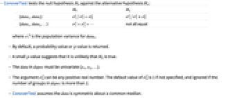
- ConoverTestは,帰無仮説
と対立仮説
で検定を行う. -


{data1,data2} 

{data1,data2,…} 

すべてが等しいわけではない - ただし,σi2は dataiの母分散である.
- デフォルトで,確率値すなわち
値が返される.
値が小さければ
が真である可能性は低い.- dspec 中の data は一変量{x1,x2,…}でなければならない.
- 引数
は任意の正の実数でよい.特に指定されていない限り
のデフォルト値は1であり,dspec 内のグループ数が2よりも多い場合は無視される. - ConoverTestは data が共通の中央値について対称であると仮定する.
- ConoverTest[data,
,"HypothesisTestData"]は htd["property"]の形で追加的な検定結果と特性の抽出に利用できるHypothesisTestDataオブジェクト htd を返す. - ConoverTest[data,
,"property"]を使って直接"property"の値を与えることができる. - 検定結果のレポートに関連する特性
-
"PValue"
値のリスト"PValueTable"
値のフォーマットされた表"ShortTestConclusion" 検定結果の簡単な説明 "TestConclusion" 検定結果の説明 "TestData" 検定統計と
値のペアのリスト"TestDataTable"
値と検定統計のフォーマットされた表"TestStatistic" 検定統計のリスト "TestStatisticTable" 検定統計のフォーマットされた表 - 検定統計はサンプル中央値からの絶対偏差の順位の平方に基づく.
- サンプル数が
個,つまり datai={xi,1,xi,2,…,xi,ni}で
の場合,値 xi,jの順位 ri,jはすべての要素 {zi,j}1≤i≤k,1≤j≤ni中の zi,jの順位である.ただし,zi,j=Abs[xi,j-Median[datai]].検定統計は,
が2の場合は
で,
が2より大きい場合は
で与えられる.ただし,
,
かつ
である.
の下で,ConoverTestの検定統計は,
が2のときはNormalDistribution[0,1]に,
が2より大きいときはChiSquareDistribution[k-1]に従うと仮定される.- ConoverTestは二乗順位検定と呼ばれることもあり,dataiが正規分布に従っていない場合にはFisherRatioTestの代りとなる.
- 使用可能なオプション
-
AlternativeHypothesis "Unequal" 対立仮説のための不等式 SignificanceLevel 0.05 診断とレポートのための切捨て VerifyTestAssumptions Automatic どの診断検定を実行するのかを設定する - ConoverTestでは,
のときにのみ
が棄却されるような切捨て
が選ばれる."TestConclusion"および"ShortTestConclusion"特性に使われる
の値はSignificanceLevelオプションで制御される.値
は対称性の検定を含む仮定の診断検定にも使われる.デフォルトで
は0.05に設定される. - ConoverTestにおけるVerifyTestAssumptionsの名前付き設定
-
"Symmetry" すべてのデータが対称であることを検証する
例題
すべて開く すべて閉じる例 (2)
data = RandomVariate[LaplaceDistribution[1, 2], {2, 100}];ConoverTest[data]さらに特性を抽出するためにHypothesisTestDataオブジェクトを作る:

ℋ = ConoverTest[data, Automatic, "HypothesisTestData"]ℋ["Properties"]data1 = RandomVariate[NormalDistribution[0, 1], 100];
data2 = RandomVariate[NormalDistribution[0, 2.5], 250];ConoverTest[{data1, data2}, 1 / 4, "TestDataTable"]Variance[data1] / Variance[data2]ConoverTest[{data1, data2}, 1 / 4, AlternativeHypothesis -> "Less"]スコープ (8)
検定 (6)
data1 = RandomVariate[NormalDistribution[0, 3], 500];
data2 = RandomVariate[NormalDistribution[1, 3], 500];ConoverTest[{data1, data2}]sample = Table[Quiet@ConoverTest[{RandomVariate[NormalDistribution[0, 3], 100], RandomVariate[NormalDistribution[1, 3], 100]}], {5 10 ^ 3}];Histogram[sample, Automatic, PDF]data3 = RandomVariate[NormalDistribution[10, 1], 350];ConoverTest[{data1, data3}]data1 = RandomVariate[NormalDistribution[0, 2], 500];
data2 = RandomVariate[NormalDistribution[0, 1], 500];Subscript[σ, 0] = 4;ConoverTest[{data1, data2}, Subscript[σ, 0]]ConoverTest[{data2, data1}, 1 / Subscript[σ, 0]]ConoverTest[{data2, data1}, Subscript[σ, 0]]data1 = RandomVariate[NormalDistribution[10, 1], 500];
data2 = RandomVariate[NormalDistribution[0, 1], 200];
data3 = RandomVariate[NormalDistribution[-3, 1], 400];ConoverTest[{data1, data2, data3}]繰り返し特性を抽出するためにHypothesisTestDataオブジェクトを作成する:
data = RandomVariate[NormalDistribution[], {2, 10^4}];ℋ = ConoverTest[data, 1, "HypothesisTestData"];ℋ["Properties"]HypothesisTestDataオブジェクトから特性をいくつか抽出する:
data = RandomVariate[NormalDistribution[], {2, 10^4}];ℋ = ConoverTest[data, 1, "HypothesisTestData"];ℋ["PValue"]ℋ["TestStatistic"]data = RandomVariate[NormalDistribution[], {2, 100}];ℋ = ConoverTest[data, 1, "HypothesisTestData"];ℋ["PValue", "TestStatistic"]レポート (2)
data = RandomVariate[NormalDistribution[], {2, 10^3}];ℋ = ConoverTest[data, 1, "HypothesisTestData"];ℋ["TestDataTable"]ℋ["TestData"]data = RandomVariate[NormalDistribution[], {3, 10^4}];ℋ = ConoverTest[data, 1, "HypothesisTestData"];ℋ["PValueTable"]ℋ["PValue"]ℋ["TestStatisticTable"]ℋ["TestStatistic"]オプション (6)
AlternativeHypothesis (3)

data = RandomVariate[NormalDistribution[], {2, 100}];ConoverTest[data, 1, AlternativeHypothesis -> "Unequal"]ConoverTest[data, 1, AlternativeHypothesis -> Automatic]両側検定を行う.あるいは2つの片側検定のうちの1つを代りに行う:
data1 = RandomVariate[NormalDistribution[0, 1], 100];
data2 = RandomVariate[NormalDistribution[0, 1.5], 100];Variance[data1] / Variance[data2]ConoverTest[{data1, data2}, 1, AlternativeHypothesis -> "Unequal"]ConoverTest[{data1, data2}, 1, AlternativeHypothesis -> "Less"]ConoverTest[{data1, data2}, 1, AlternativeHypothesis -> "Greater"]data1 = RandomVariate[NormalDistribution[0, .9], 100];
data2 = RandomVariate[NormalDistribution[0, 1], 100];Variance[data1] / Variance[data2]ConoverTest[{data1, data2}, .75, AlternativeHypothesis -> "Less"]ConoverTest[{data1, data2}, 1.5, AlternativeHypothesis -> "Less"]SignificanceLevel (1)
有意水準は"TestConclusion"と"ShortTestConclusion"に使われる:
data = BlockRandom[SeedRandom[1];RandomVariate[NormalDistribution[0, 1], {2, 100}]];ℋ1 = ConoverTest[data, 2, "HypothesisTestData", SignificanceLevel -> .05];ℋ2 = ConoverTest[data, 2, "HypothesisTestData", SignificanceLevel -> .01];ℋ1["TestConclusion"]ℋ2["TestConclusion"]ℋ1["ShortTestConclusion"]ℋ2["ShortTestConclusion"]VerifyTestAssumptions (2)
診断は,AllあるいはNoneを使ってまとめて制御することができる:
BlockRandom[SeedRandom[4];data1 = RandomVariate[ExponentialDistribution[1 / Sqrt[3]], 1000];
data2 = RandomVariate[NormalDistribution[0, Sqrt[3]], 1000]];ConoverTest[{data1, data2}, 1 / 4, VerifyTestAssumptions -> All]
ConoverTest[{data1, data2}, 1 / 4, VerifyTestAssumptions -> None]BlockRandom[SeedRandom[2];data1 = RandomVariate[ExponentialDistribution[1 / Sqrt[3]], 1000];
data2 = RandomVariate[NormalDistribution[0, Sqrt[3]], 1000]];ConoverTest[{data1, data2}, 1 / 4, VerifyTestAssumptions -> "Symmetry"]
対称性の仮定をTrueに設定する:
ConoverTest[{data1, data2}, 1 / 4, VerifyTestAssumptions -> "Symmetry" -> True]アプリケーション (1)
1990年代の前半と後半において,S&P 500の日々の点の変化の分散を比べる:
sp90to95 = FinancialData["SP500", {{1990, 1}, {1994, 12, 31}}];
sp95to00 = FinancialData["SP500", {{1995, 1}, {1999, 12, 31}}];DateListPlot[{sp90to95, sp95to00}]DistributionFitTest /@ {spA = Differences[sp90to95], spB = Differences[sp95to00]}SmoothHistogram[{spA, spB}, PlotRange -> All]ConoverTest[{spA, spB}, 1, "TestDataTable"]特性と関係 (8)
グループ数が2のとき,検定統計は
の下でNormalDistribution[0,1]に従う:
data1 = RandomVariate[NormalDistribution[-5, 1], {1000, 100}];
data2 = RandomVariate[NormalDistribution[3, 1], {1000, 400}];T = MapThread[ConoverTest[{#1, #2}, Automatic, "TestStatistic", VerifyTestAssumptions -> None]&, {data1, data2}];Show[Plot[PDF[NormalDistribution[], x], {x, -4, 4}], SmoothHistogram[T, PlotStyle -> Orange]]DistributionFitTest[T, NormalDistribution[]]グループ数が
(
)のとき,検定統計は
の下でChiSquareDistribution[k-1]に従う:
data1 = RandomVariate[NormalDistribution[-5, 1], {2000, 600}];
data2 = RandomVariate[NormalDistribution[3, 1], {2000, 500}];
data3 = RandomVariate[NormalDistribution[2, 1], {2000, 400}];T = MapThread[ConoverTest[{#1, #2, #3}, Automatic, "TestStatistic", VerifyTestAssumptions -> None]&, {data1, data2, data3}];Show[Histogram[T, Automatic, "PDF"], Plot[PDF[ChiSquareDistribution[2], x], {x, 0, 8}]]DistributionFitTest[T, ChiSquareDistribution[2]]FisherRatioTestと違って,Conover検定は正規性を仮定しない:
data1 = RandomVariate[LaplaceDistribution[1, 2], {1000, 100}];
data2 = RandomVariate[LaplaceDistribution[1, 2], {1000, 75}];fisher = MapThread[FisherRatioTest[{#1, #2}, Automatic, VerifyTestAssumptions -> None]&, {data1, data2}];conover = MapThread[ConoverTest[{#1, #2}, Automatic, VerifyTestAssumptions -> None]&, {data1, data2}];FisherRatioTestの結果は,
値を過小評価する:
Histogram[{fisher, conover}, Automatic, "PDF"]Conover検定は,データが共通の中央値について対称であると仮定する:
data1 = RandomVariate[d1 = NormalDistribution[0, ((25/6))^1 / 2], {1000, 50}];
data2 = RandomVariate[d2 = TriangularDistribution[{-10, 0}], {1000, 50}];Variance[d1] == Variance[d2]T = MapThread[ConoverTest[{#1, #2}, Automatic, "TestStatistic", VerifyTestAssumptions -> None]&, {data1, data2}];Show[Plot[PDF[NormalDistribution[], x], {x, -4, 4}], SmoothHistogram[T, PlotStyle -> Orange]]検定統計の分布は,データが非対称である場合,標準正規分布に従わない:
DistributionFitTest[T, NormalDistribution[]]ConoverTestの検定統計は順位に基づく:
n = 1000;m = 750;Subscript[σ, 0] = 2;data1 = RandomVariate[NormalDistribution[1, Sqrt[6]], n];
data2 = RandomVariate[StudentTDistribution[3], m];同順位のものがなければ,Orderingを使って順位を計算することができる:
ranks = Ordering[Ordering[Join[Abs[data1 - Median[data1]], Sqrt[Subscript[σ, 0]] Abs[data2 - Median[data2]]]]];R2 = (1/n + m)Underoverscript[∑, i = 1, n + m]ranks[[i]]^2;R4 = Underoverscript[∑, i = 1, n + m]ranks[[i]]^4;(Underoverscript[∑, i = 1, n]ranks[[i]]^2 - n R2) / Sqrt[(m n (-(m + n) R2^2 + R4)/(-1 + m + n) (m + n))]//NConoverTest[{data1, data2}, Subscript[σ, 0], "TestStatistic"]PearsonChiSquareTestを使って,共通の中央値においてデータの対称性を検定する:
data1 = RandomVariate[NormalDistribution[10, 1], 100];
data2 = RandomVariate[NormalDistribution[3, 2], 150];
data3 = RandomVariate[ExponentialDistribution[10], 135];SymmTest[d1_, d2_] := Block[{d = Sort[Flatten[{d1 - Median[d1], d2 - Median[d2]}]], c, symmDat}, c = Ceiling[(Length[d]/2)];symmDat = Join[d[[1 ;; c]], -d[[1 ;; c]]];PearsonChiSquareTest[symmDat, d]]SymmTest[data1, data2]ConoverTest[{data1, data2}, 1, "TestDataTable", VerifyTestAssumptions -> "Symmetry"]SymmTest[data2, data3]警告メッセージの
値は,PearsonChiSquareTestのそれに一致する:
ConoverTest[{data2, data3}, 1, "TestDataTable", VerifyTestAssumptions -> "Symmetry"]Conover検定は,入力がTimeSeriesのときはタイムスタンプを無視する:
ts1 = TemporalData[TimeSeries, {{{1.224578634529677, 0.47929635789978015, 0.6572781300178168,
0.21496048742669355, 0.7299608014554928, -0.2495111111278263, -1.3286551762002712,
0.552725018274874, 0.19272112205837066, 1.1809144012420882, -1.1671 ... 40938613662046, 1.052394590214582, 0.9345044123980388, 0.38537803109557855,
-0.48660931166089394, -0.71203560340161}}, {{0, 100, 1}}, 1, {"Continuous", 1},
{"Discrete", 1}, 1, {ValueDimensions -> 1, ResamplingMethod -> None}}, False, 10.1];ts2 = TemporalData[TimeSeries, {{{-1.2160757838495546, 0.5212591188357838, -0.0932747538180776,
-2.306367634798702, -2.5366722726947994, -0.7924813212437647, -2.65435901675047,
-1.1098678592653723, -0.7814091835518528, -1.9685555851254093, -0.0 ... 1001061264, -0.1887471329804458, -2.0547107874294928, -1.3896240275653011,
-0.5073077090484948, 0.13302942350391606}}, {{0, 100, 1}}, 1, {"Continuous", 1},
{"Discrete", 1}, 1, {ValueDimensions -> 1, ResamplingMethod -> None}}, False, 10.1];ConoverTest[{ts1, ts2}]ConoverTest[{ts1["Values"], ts2["Values"]}]Conover検定はTemporalDataの経路構造を認識する:
td = TemporalData[Automatic, {{{1.224578634529677, 0.47929635789978015, 0.6572781300178168,
0.21496048742669355, 0.7299608014554928, -0.2495111111278263, -1.3286551762002712,
0.552725018274874, 0.19272112205837066, 1.1809144012420882, -1.16711 ... 01061264, -0.1887471329804458, -2.0547107874294928,
-1.3896240275653011, -0.5073077090484948, 0.13302942350391606}}, {{0, 100, 1}}, 2,
{"Continuous", 2}, {"Discrete", 1}, 1, {ValueDimensions -> 1, ResamplingMethod -> None}}, False,
10.1];ConoverTest[td]ConoverTest[td["ValueList"]]考えられる問題 (3)
data1 = RandomVariate[NormalDistribution[], 1000];
data2 = RandomVariate[NormalDistribution[10, 1], 1000];
data3 = RandomVariate[ParetoDistribution[1, 2], 1000];位置のシフトを考慮に入れると,最初の2つのデータ集合は対称である:
SmoothHistogram[Join[data1 - Median[data1], data2 - Median[data2]]]ConoverTest[{data1, data2}, VerifyTestAssumptions -> "Symmetry"]SmoothHistogram[Join[data2 - Median[data2], data3 - Median[data3]], PlotRange -> All]ConoverTest[{data2, data3}, VerifyTestAssumptions -> "Symmetry"]
グループ数が2より多いとき,Conover検定は引数
を無視する:
data = RandomVariate[NormalDistribution[1, 2], {4, 100}];Length[data]ConoverTest[data, 2, "TestDataTable"]データ内に2より多いグループがある場合,Conover検定は対立仮説として両側検定しか認めない:
data = RandomVariate[NormalDistribution[1, 2], {4, 100}];ConoverTest[data, 1, AlternativeHypothesis -> "Unequal"]ConoverTest[data, 1, AlternativeHypothesis -> "Greater"]ConoverTest[data, 1, AlternativeHypothesis -> "Less"]おもしろい例題 (1)
data1 = RandomVariate[NormalDistribution[], {250, 100}];
data2 = RandomVariate[NormalDistribution[], {250, 100}];T1 = MapThread[ConoverTest[{#1, #2}, 1, "TestStatistic"]&, {data1, data2}];T2 = MapThread[ConoverTest[{#1, #2}, 2, "TestStatistic"]&, {data1, data2}];SmoothHistogram[{T1, T2}, Filling -> Axis, PlotLegends -> {"SubscriptBox[H, 0] is True", "SubscriptBox[H, 0] is False"}]関連するガイド
-
▪
- 仮説検定
テキスト
Wolfram Research (2010), ConoverTest, Wolfram言語関数, https://reference.wolfram.com/language/ref/ConoverTest.html (2017年に更新).
CMS
Wolfram Language. 2010. "ConoverTest." Wolfram Language & System Documentation Center. Wolfram Research. Last Modified 2017. https://reference.wolfram.com/language/ref/ConoverTest.html.
APA
Wolfram Language. (2010). ConoverTest. Wolfram Language & System Documentation Center. Retrieved from https://reference.wolfram.com/language/ref/ConoverTest.html
BibTeX
@misc{reference.wolfram_2026_conovertest, author="Wolfram Research", title="{ConoverTest}", year="2017", howpublished="\url{https://reference.wolfram.com/language/ref/ConoverTest.html}", note=[Accessed: 14-September-2026]}
BibLaTeX
@online{reference.wolfram_2026_conovertest, organization={Wolfram Research}, title={ConoverTest}, year={2017}, url={https://reference.wolfram.com/language/ref/ConoverTest.html}, note=[Accessed: 14-September-2026]}