-
See Also
- EstimatedDistribution
- FindDistributionParameters
- HypothesisTestData
- LocationTest
- VarianceTest
- IndependenceTest
- LogRankTest
- AndersonDarlingTest
- KolmogorovSmirnovTest
- CramerVonMisesTest
- JarqueBeraALMTest
- KuiperTest
- MardiaCombinedTest
- MardiaKurtosisTest
- MardiaSkewnessTest
- BaringhausHenzeTest
- PearsonChiSquareTest
- ShapiroWilkTest
- WatsonUSquareTest
- Related Guides
-
-
See Also
- EstimatedDistribution
- FindDistributionParameters
- HypothesisTestData
- LocationTest
- VarianceTest
- IndependenceTest
- LogRankTest
- AndersonDarlingTest
- KolmogorovSmirnovTest
- CramerVonMisesTest
- JarqueBeraALMTest
- KuiperTest
- MardiaCombinedTest
- MardiaKurtosisTest
- MardiaSkewnessTest
- BaringhausHenzeTest
- PearsonChiSquareTest
- ShapiroWilkTest
- WatsonUSquareTest
- Related Guides
-
See Also
DistributionFitTest[data]
tests whether data is normally distributed.
DistributionFitTest[data,dist]
tests whether data is distributed according to dist.
DistributionFitTest[data,dist,"property"]
returns the value of "property".


DistributionFitTest
DistributionFitTest[data]
tests whether data is normally distributed.
DistributionFitTest[data,dist]
tests whether data is distributed according to dist.
DistributionFitTest[data,dist,"property"]
returns the value of "property".
Details and Options


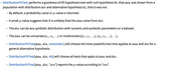
- DistributionFitTest performs a goodness-of-fit hypothesis test with null hypothesis
 that data was drawn from a population with distribution dist and alternative hypothesis
  that it was not.
 - By default, a probability value or
 -value is returned.
 - A small
 -value suggests that it is unlikely that the data came from dist.
 - The dist can be any symbolic distribution with numeric and symbolic parameters or a dataset.
- The data can be univariate {x1,x2,…} or multivariate {{x1,y1,…},{x2,y2,…},…}.
- DistributionFitTest[data,dist,Automatic] will choose the most powerful test that applies to data and dist for a general alternative hypothesis.
- DistributionFitTest[data,dist,All] will choose all tests that apply to data and dist.
- DistributionFitTest[data,dist,"test"] reports the
 -value according to "test".
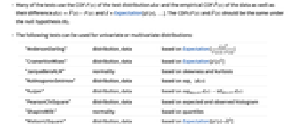
 - Many of the tests use the CDF
 of the test distribution dist and the empirical CDF
  of the data as well as their difference
  and
and  =Expectation[d(x),…]. The CDFs
  and
and  should be the same under the null hypothesis
  .
. - The following tests can be used for univariate or multivariate distributions:
-
"AndersonDarling" distribution, data based on Expectation[  ]
]"CramerVonMises" distribution, data based on Expectation[d(x)2] "JarqueBeraALM" normality based on skewness and kurtosis "KolmogorovSmirnov" distribution, data based on ![sup_x TemplateBox[{{d, (, x, )}}, Abs] sup_x TemplateBox[{{d, (, x, )}}, Abs]](Files/DistributionFitTest.en/14.png)
"Kuiper" distribution, data based on 
"PearsonChiSquare" distribution, data based on expected and observed histogram "ShapiroWilk" normality based on quantiles "WatsonUSquare" distribution, data based on Expectation[  ]
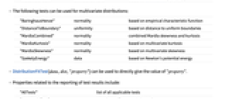
] - The following tests can be used for multivariate distributions:
-
"BaringhausHenze" normality based on empirical characteristic function "DistanceToBoundary" uniformity based on distance to uniform boundaries "MardiaCombined" normality combined Mardia skewness and kurtosis "MardiaKurtosis" normality based on multivariate kurtosis "MardiaSkewness" normality based on multivariate skewness "SzekelyEnergy" data based on Newton's potential energy - DistributionFitTest[data,dist,"property"] can be used to directly give the value of "property".
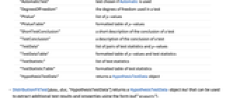
- Properties related to the reporting of test results include:
-
"AllTests" list of all applicable tests "AutomaticTest" test chosen if Automatic is used "DegreesOfFreedom" the degrees of freedom used in a test "PValue" list of  -values
"PValueTable" formatted table of  -values
"ShortTestConclusion" a short description of the conclusion of a test "TestConclusion" a description of the conclusion of a test "TestData" list of pairs of test statistics and  -values
"TestDataTable" formatted table of  -values and test statistics
"TestStatistic" list of test statistics "TestStatisticTable" formatted table of test statistics "HypothesisTestData" returns a HypothesisTestData object - DistributionFitTest[data,dist,"HypothesisTestData"] returns a HypothesisTestData object htd that can be used to extract additional test results and properties using the form htd["property"].
- Properties related to the data distribution include:
-
"FittedDistribution" fitted distribution of data "FittedDistributionParameters" distribution parameters of data - The following options can be given:
-
Method Automatic the method to use for computing  -values
SignificanceLevel 0.05 cutoff for diagnostics and reporting - For a test for goodness of fit, a cutoff
 is chosen such that
  is rejected only if
  . The value of
  used for the "TestConclusion" and "ShortTestConclusion" properties is controlled by the SignificanceLevel option. By default,
  is set to 0.05.
 - With the setting Method->"MonteCarlo",
 datasets of the same length as the input si are generated under
  using the fitted distribution. The EmpiricalDistribution from DistributionFitTest[si,dist,{"TestStatistic",test}] is then used to estimate the
  -value.
Examples
open all close allBasic Examples (3)
Create a HypothesisTestData object for further property extraction:
Compare the histogram of the data to the PDF of the test distribution:
Test the fit of a set of data to a particular distribution:
Extract the Anderson–Darling test table:
Verify the test results with ProbabilityPlot:
Test data for goodness of fit to a multivariate distribution:
Plot the marginal PDFs of the test distribution against the data to confirm the test results:
Scope (22)
Testing (16)
The ![]() -values for the normally distributed data are typically large:
-values for the normally distributed data are typically large:
The ![]() -values for data that is not normally distributed are typically small:
-values for data that is not normally distributed are typically small:
Set the third argument to Automatic to apply a generally powerful and appropriate test:
The property "AutomaticTest" can be used to determine which test was chosen:
Test whether data fits a particular distribution:
There is insufficient evidence to reject a good fit to a WeibullDistribution[1,2]:
Test for goodness of fit to a derived distribution:
The ![]() -value is large for the mixture data compared to data not drawn from the mixture:
-value is large for the mixture data compared to data not drawn from the mixture:
Test for goodness of fit for quantity data:
Check goodness-of-fit for a specific distribution:
Test for goodness of fit to a formula-based distribution:
Unspecified parameters will be estimated from the data:
The ![]() -value is dependent on which parameters were estimated:
-value is dependent on which parameters were estimated:
Test some data for multivariate normality:
The ![]() -values for normally distributed data are typically large compared to non-normal data:
-values for normally distributed data are typically large compared to non-normal data:
Test some data for goodness of fit to a particular multivariate distribution:
Test a MultinormalDistribution and multivariate UniformDistribution, respectively:
Compare the distributions of two datasets:
The sample sizes need not be equal:
Compare the distributions of two multivariate datasets:
The ![]() -values for equally distributed data are large compared to unequally distributed data:
-values for equally distributed data are large compared to unequally distributed data:
Perform a particular goodness-of-fit test:
Any number of tests can be performed simultaneously:
Perform all tests, appropriate to the data and distribution, simultaneously:
Use the property "AllTests" to identify which tests were used:
Create a HypothesisTestData object for repeated property extraction:
The properties available for extraction:
Extract some properties from a HypothesisTestData object:
The ![]() -value and test statistic from a Cramér–von Mises test:
-value and test statistic from a Cramér–von Mises test:
Extract any number of properties simultaneously:
The results from the Anderson–Darling ![]() -value and test statistic:
-value and test statistic:
Data Properties (2)
Obtain the fitted distribution when parameters have been unspecified:
Extract the parameters from the fitted distribution:
Plot the PDF of the fitted distribution against the data:
Confirm the fit with a goodness-of-fit test:
The test distribution is returned when the parameters have been specified:
Reporting (4)
Tabulate the results from a selection of tests:
A full table of all appropriate test results:
A table of selected test results:
Retrieve the entries from a test table for customized reporting:
The ![]() -values are above 0.05, so there is not enough evidence to reject normality at that level:
-values are above 0.05, so there is not enough evidence to reject normality at that level:
Tabulate ![]() -values for a test or group of tests:
-values for a test or group of tests:
A table of ![]() -values from all appropriate tests:
-values from all appropriate tests:
A table of ![]() -values from a subset of tests:
-values from a subset of tests:
Report the test statistic from a test or group of tests:
Options (6)
Method (4)
Use Monte Carlo-based methods, or choose the fastest method automatically:
Set the number of samples to use for Monte Carlo-based methods:
The Monte Carlo estimate converges to the true ![]() -value with increasing samples:
-value with increasing samples:
Set the random seed used in Monte Carlo-based methods:
The seed affects the state of the generator and has some effect on the resulting ![]() -value:
-value:
Monte Carlo simulations generate many test statistics under ![]() :
:
The estimated distribution of the test statistics under ![]() :
:
The empirical estimate of the ![]() -value agrees with the Monte Carlo estimate:
-value agrees with the Monte Carlo estimate:
Applications (12)
Analyze whether a dataset is drawn from a normal distribution:
Perform a series of goodness-of-fit tests:
Visually compare the empirical and theoretical CDFs in a QuantilePlot:
Visually compare the empirical CDF to that of the test distribution:
Determine whether snowfall accumulations in Buffalo are normally distributed:
Use the Jarque–Bera ALM test and Shapiro–Wilk test to assess normality:
The SmoothHistogram agrees with the test results:
The QuantilePlot suggests a reasonably good fit:
Use a goodness-of-fit test to verify the fit suggested by visualization such as a histogram:
The Kolmogorov–Smirnov test agrees with the good fit suggested in the histogram:
Test whether the absolute magnitudes of the 100 brightest stars are normally distributed:
The value of the statistic and p-value for the automatic test:
Test whether multivariate data is uniformly distributed over a box:
Use the distance-to-boundary test:
Use Szekely's energy test to compare two multivariate datasets:
The distributions for measures of counterfeit and genuine notes are significantly different:
Visually compare the marginal distributions to determine the origin of the discrepancy:
Test whether data is uniformly distributed on a unit circle:
Kuiper's test and the Watson ![]() test are useful for testing uniformity on a circle:
test are useful for testing uniformity on a circle:
The first dataset is randomly distributed, the second is clustered:
Determine if a model is appropriate for day-to-day point changes in the S&P 500 index:
The histogram suggests a heavy-tailed, symmetric distribution:
Try a LaplaceDistribution:
For very large datasets, small deviations from the test distribution are readily detected:
Test the residuals from a LinearModelFit for normality:
The Shapiro–Wilk test suggests that the residuals are not normally distributed:
The QuantilePlot suggests large deviations in the left tail of the distribution:
Simulate the distribution of a test statistic to obtain a Monte Carlo ![]() -value:
-value:
Visualize the distribution of the test statistic using SmoothHistogram:
Obtain the Monte Carlo ![]() -value from an Anderson–Darling test:
-value from an Anderson–Darling test:
Compare with the ![]() -value returned by DistributionFitTest:
-value returned by DistributionFitTest:
Obtain an estimate of the power for a hypothesis test:
Visualize the approximate power curve:
Estimate the power of the Shapiro–Wilk test when the underlying distribution is a StudentTDistribution[2], the test size is 0.05, and the sample size is 35:
Smoothing a dataset using kernel density estimation can remove noise while preserving the structure of the underlying distribution of the data. Here two datasets are created from the same distribution:
The unsmoothed data provides a noisy estimate of the underlying distributions:
Noise would lead to committing a type I error:
Smoothing reduces the noise and results in a correct conclusion at the 5% level:
Properties & Relations (16)
By default, univariate data is compared to a NormalDistribution:
The parameters of the distribution are estimated from the data:
Multivariate data is compared to a MultinormalDistribution by default:
Unspecified parameters of the distribution are estimated from the data:
Maximum likelihood estimates are used for unspecified parameters of the test distribution:
The ![]() -value suggests the expected proportion of false positives (type I errors):
-value suggests the expected proportion of false positives (type I errors):
Setting the size of a test to 0.05 results in an erroneous rejection of ![]() about 5% of the time:
about 5% of the time:
Type II errors arise when ![]() is not rejected, given it is false:
is not rejected, given it is false:
Increasing the size of the test lowers the type II error rate:
The ![]() -value for a valid test has a UniformDistribution[{0,1}] under
-value for a valid test has a UniformDistribution[{0,1}] under ![]() :
:
Verify the uniformity using the Kolmogorov–Smirnov test:
The power of each test is the probability of rejecting ![]() when it is false:
when it is false:
Under these conditions, the Pearson ![]() test has the lowest power:
test has the lowest power:
The power of each test decreases with sample size:
Some tests perform better than others with small sample sizes:
Some tests are more powerful than others for detecting differences in location:
Some tests are more powerful than others for detecting differences in scale:
The Pearson ![]() test requires large sample sizes to have high power:
test requires large sample sizes to have high power:
Some tests perform better than others when testing normality:
The Jarque–Bera ALM and Shapiro–Wilk tests are the most powerful for small samples:
Tests designed for the composite hypothesis of normality ignore specified parameters:
Different tests examine different properties of the distribution. Conclusions based on a particular test may not always agree with those based on another test:
The green region represents a correct conclusion by both tests. Points fall in the red region when a type II error is committed by both tests. The gray region shows where the tests disagree:
Estimating parameters prior to testing affects the distribution of the test statistic:
The distribution of the test statistics and resulting ![]() -values under
-values under ![]() :
:
Failing to account for the estimation leads to an overestimate of ![]() -values:
-values:
The distribution fit test works with the values only when the input is a TimeSeries:
Possible Issues (5)
Some tests require that the parameters be prespecified and not estimated for valid ![]() -values:
-values:
It is usually possible to use Monte Carlo methods to arrive at a valid ![]() -value:
-value:
For many distributions, corrections are applied when parameters are estimated:
The Jarque–Bera ALM test must have sample sizes of at least 10 for valid ![]() -values:
-values:
Use Monte Carlo methods to arrive at a valid ![]() -value:
-value:
The Kolmogorov–Smirnov test and Kuiper's test expect no ties in the data:
The Jarque–Bera ALM test and Shapiro–Wilk test are only valid for testing normality:
Careful interpretation is required when some tests are used for discrete distributions:
The Pearson ![]() test applies directly for discrete distributions:
test applies directly for discrete distributions:
See Also
EstimatedDistribution FindDistributionParameters HypothesisTestData LocationTest VarianceTest IndependenceTest LogRankTest AndersonDarlingTest KolmogorovSmirnovTest CramerVonMisesTest JarqueBeraALMTest KuiperTest MardiaCombinedTest MardiaKurtosisTest MardiaSkewnessTest BaringhausHenzeTest PearsonChiSquareTest ShapiroWilkTest WatsonUSquareTest
Text
Wolfram Research (2010), DistributionFitTest, Wolfram Language function, https://reference.wolfram.com/language/ref/DistributionFitTest.html (updated 2015).
CMS
Wolfram Language. 2010. "DistributionFitTest." Wolfram Language & System Documentation Center. Wolfram Research. Last Modified 2015. https://reference.wolfram.com/language/ref/DistributionFitTest.html.
APA
Wolfram Language. (2010). DistributionFitTest. Wolfram Language & System Documentation Center. Retrieved from https://reference.wolfram.com/language/ref/DistributionFitTest.html
BibTeX
@misc{reference.wolfram_2025_distributionfittest, author="Wolfram Research", title="{DistributionFitTest}", year="2015", howpublished="\url{https://reference.wolfram.com/language/ref/DistributionFitTest.html}", note=[Accessed: 05-May-2026]}
BibLaTeX
@online{reference.wolfram_2025_distributionfittest, organization={Wolfram Research}, title={DistributionFitTest}, year={2015}, url={https://reference.wolfram.com/language/ref/DistributionFitTest.html}, note=[Accessed: 05-May-2026]}