CoxianDistribution

✖
`CoxianDistribution`

✖

CoxianDistribution[{α₁,…,α_m-1},{λ₁,…,λ_m}]

represent an m-phase Coxian distribution with phase probabilities α_i and rates λ_i.

Details

An m-phase Coxian distribution can be interpreted as m sequential service phases with rates λ_i, where one continues to service phase i+1 with probability α_i and finishes with probability 1-α_i.
The probability density for value and distinct rates is a linear combination of exponentials for and zero for .
CoxianDistribution allows α_i to be any positive number not greater than 1 and λ_i to be any positive real numbers.
CoxianDistribution allows λ_i to be any quantities of the same unit dimensions and α_i to be dimensionless quantities. »
CoxianDistribution can be used with such functions as Mean, CDF, and RandomVariate.

Background & Context

CoxianDistribution[{α₁,…,α_m-1},{λ₁,…,λ_m}] represents a continuous statistical distribution defined over the interval , parameterized by two vectors (α₁,…,α_m-1) and (λ₁,…,λ_m), and known as an -phase Coxian distribution. The parameters α_i are called "phase probabilities" and have values in the interval , while the parameters λ_i are called "phase rates" and have positive real values. Together, these parameters determine the overall shape of the probability density function (PDF) and, depending on their values, the PDF may be monotonic decreasing or unimodal. In addition, the tails of the PDF are "thin" in the sense that the PDF decreases exponentially rather than decreasing algebraically for large values of . (This behavior can be made quantitatively precise by analyzing the SurvivalFunction of the distribution.) Random variables satisfying XCoxianDistribution[{α₁,…,α_m-1},{λ₁,…,λ_m}] are sometimes said to have a Coxian distribution of order .
While the foundations of Coxian distributions originate with the work of mathematician D. R. Cox in the 1950s, much of the current corpus of knowledge was established through work on generalizations of hyperexponential distributions dating from the 1980s. To be mathematically precise, a random variable has a Coxian distribution of order if it starts in phase 1 and goes through no more than exponential phases where, for the phase (which has mean length equal to ), continues to phase i+1 with probability α_i and finishes with probability 1-α_i. A number of real-world phenomena behave in a way naturally modeled by a Coxian distribution, including teletraffic in mobile cellular networks, durations of stay among patients in geriatric facilities, and queueing systems of various types.
RandomVariate can be used to give one or more machine- or arbitrary-precision (the latter via the WorkingPrecision option) pseudorandom variates from a Coxian distribution. Distributed[x,CoxianDistribution[{α₁,…,α_m-1},{λ₁,…,λ_m}]], written more concisely as xCoxianDistribution[{α₁,…,α_m-1},{λ₁,…,λ_m}], can be used to assert that a random variable x is distributed according to a Coxian distribution. Such an assertion can then be used in functions such as Probability, NProbability, Expectation, and NExpectation.
The probability density and cumulative distribution functions may be given using PDF[CoxianDistribution[{α₁,…,α_m-1},{λ₁,…,λ_m}],x] and CDF[CoxianDistribution[{α₁,…,α_m-1},{λ₁,…,λ_m}],x]. The mean, median, variance, raw moments, and central moments may be computed using Mean, Median, Variance, Moment, and CentralMoment, respectively.
DistributionFitTest can be used to test if a given dataset is consistent with a Coxian distribution, EstimatedDistribution to estimate a Coxian parametric distribution from given data, and FindDistributionParameters to fit data to a Coxian distribution. ProbabilityPlot can be used to generate a plot of the CDF of given data against the CDF of a symbolic Coxian distribution and QuantilePlot to generate a plot of the quantiles of given data against the quantiles of a symbolic Coxian distribution.
TransformedDistribution can be used to represent a transformed Coxian distribution, CensoredDistribution to represent the distribution of values censored between upper and lower values, and TruncatedDistribution to represent the distribution of values truncated between upper and lower values. CopulaDistribution can be used to build higher-dimensional distributions that contain a Coxian distribution, and ProductDistribution can be used to compute a joint distribution with independent component distributions involving Coxian distributions.
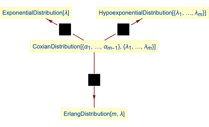
The Coxian distribution is related to a number of other distributions. For example, CoxianDistribution is related to HyperexponentialDistribution both in its derivation and in the sense that the PDF of -phase distribution CoxianDistribution[{1,…,1},{λ₁,…,λ_m}] is the same as that of ExponentialDistribution[{λ₁,…,λ_m}]. This creates a link between CoxianDistribution and ExponentialDistribution as well, and this link can be made precise by noting that the -phase CoxianDistribution[{0,…,α_m-1},{λ₁,…,λ_m}] has the same PDF as ExponentialDistribution[λ₁]. Finally, for any λ, the PDF of the -phase distribution CoxianDistribution[{1,…,1},{λ,…,λ}] is the same as that of ErlangDistribution[{m,λ}].

Examples

open allclose all

Basic Examples (4)Summary of the most common use cases

Probability density function:

In[1]:=1

✖

https://wolfram.com/xid/0e485ymvd01j0q-pjhn1b

Out[1]=1

In[2]:=2

✖

https://wolfram.com/xid/0e485ymvd01j0q-0pwyru

Out[2]=2

Cumulative distribution function:

In[1]:=1

✖

https://wolfram.com/xid/0e485ymvd01j0q-3cmr65

Out[1]=1

In[2]:=2

✖

https://wolfram.com/xid/0e485ymvd01j0q-lx3361

Out[2]=2

Mean and variance:

In[1]:=1

✖

https://wolfram.com/xid/0e485ymvd01j0q-nxa33t

Out[1]=1

In[2]:=2

✖

https://wolfram.com/xid/0e485ymvd01j0q-hflsh0

Out[2]=2

Median can be found numerically:

In[1]:=1

✖

https://wolfram.com/xid/0e485ymvd01j0q-41cr5n

Out[1]=1

Scope (8)Survey of the scope of standard use cases

Generate a sample of pseudorandom numbers from a Coxian distribution:

In[1]:=1

✖

https://wolfram.com/xid/0e485ymvd01j0q-tscvhm

Compare the histogram to the PDF:

In[2]:=2

✖

https://wolfram.com/xid/0e485ymvd01j0q-fw0ala

Out[2]=2

Distribution parameters estimation:

In[1]:=1

✖

https://wolfram.com/xid/0e485ymvd01j0q-45b7g2

Estimate the distribution parameters from sample data:

In[2]:=2

✖

https://wolfram.com/xid/0e485ymvd01j0q-epi747

Out[2]=2

Compare a density histogram of the sample with the PDF of the estimated distribution:

In[3]:=3

✖

https://wolfram.com/xid/0e485ymvd01j0q-f8ui5o

Out[3]=3

Skewness:

In[1]:=1

✖

https://wolfram.com/xid/0e485ymvd01j0q-eiql9h

Out[1]=1

In[2]:=2

✖

https://wolfram.com/xid/0e485ymvd01j0q-fmqn15

Out[2]=2

Kurtosis:

In[1]:=1

✖

https://wolfram.com/xid/0e485ymvd01j0q-z8ruhw

Out[1]=1

In[2]:=2

✖

https://wolfram.com/xid/0e485ymvd01j0q-j1nw9k

Out[2]=2

Different moments with closed forms as functions of parameters:

In[1]:=1

✖

https://wolfram.com/xid/0e485ymvd01j0q-js043h

Moment:

In[2]:=2

✖

https://wolfram.com/xid/0e485ymvd01j0q-rx074o

Out[2]=2

CentralMoment:

In[3]:=3

✖

https://wolfram.com/xid/0e485ymvd01j0q-pknsqa

Out[3]=3

FactorialMoment:

In[4]:=4

✖

https://wolfram.com/xid/0e485ymvd01j0q-zg9ct4

Out[4]=4

Cumulant:

In[5]:=5

✖

https://wolfram.com/xid/0e485ymvd01j0q-9gzmth

Out[5]=5

Hazard function:

In[1]:=1

✖

https://wolfram.com/xid/0e485ymvd01j0q-0gsst0

Out[1]=1

In[2]:=2

✖

https://wolfram.com/xid/0e485ymvd01j0q-1ri4li

Out[2]=2

Quantile function:

In[1]:=1

✖

https://wolfram.com/xid/0e485ymvd01j0q-txywq

Out[1]=1

Consistent use of Quantity in parameters yields QuantityDistribution:

In[1]:=1

✖

https://wolfram.com/xid/0e485ymvd01j0q-iwn5xx

Out[1]=1

Find the median time:

In[2]:=2

✖

https://wolfram.com/xid/0e485ymvd01j0q-vckn5

Out[2]=2

In[3]:=3

✖

https://wolfram.com/xid/0e485ymvd01j0q-97d2q

Out[3]=3

Applications (2)Sample problems that can be solved with this function

A customer enters a feed-forward queueing system with two service locations that have exponential service times with rates of 25 and 28 customers per hour, respectively. After being serviced at the first location, the customer prematurely leaves the system with probability of ; otherwise, the customer proceeds to the next service location. Find the probability that the customer is in the system for more than 5 minutes:

In[1]:=1

✖

https://wolfram.com/xid/0e485ymvd01j0q-c5qd3

Out[1]=1

In[2]:=2

✖

https://wolfram.com/xid/0e485ymvd01j0q-hixxsn

Out[2]=2

In[3]:=3

✖

https://wolfram.com/xid/0e485ymvd01j0q-e42t58

Out[3]=3

The first passage time of the continuous Markov chain into the only absorbing state, having started in a transient state, is generally described by a mixture of Coxian distributions:

In[1]:=1