




RipleyK


更多信息和选项
- 积
 ,其中
 为平均密度,给出期望位于点 r 距离范围内的点数,不计算点本身.
-
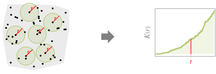
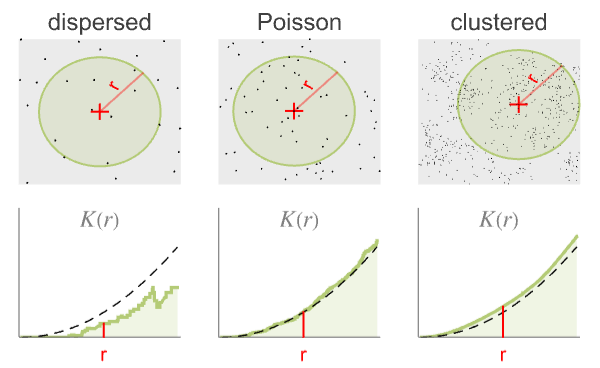
- RipleyK 测量半径 r 内的点的空间均匀性. 与泊松点过程相比的结果为:
-
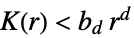
比泊松点过程更分散 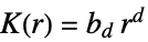
与泊松点过程相似,即具有完全空间随机性 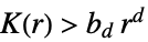
比泊松点过程聚类性更强 - 下面,
 是
 中单位球体的体积.
-
- 半径 r 可以是单个值或值的列表. 如果没有指定 r,RipleyK 会返回一个 PointStatisticFunction,可用其重复计算
 函数.
- 可用以下形式给出点 pdata:
-
{p1,p2,…} 点 pi GeoPosition[…],GeoPositionXYZ[…],… 地理点 SpatialPointData[…] 空间点集 {pts,reg} 点集 pts 和观察区域 reg - 如果没有给出观察区域 reg,则用 RipleyRassonRegion 自动计算区域.
- 可用以下形式给出点过程 pproc:
-
proc 点过程 proc {proc,reg} 点过程 proc 和观察区域 reg - 观察区域 reg 不应含有参数且 SpatialObservationRegionQ 的结果为真.
- 已分组数据 bdata 来自 SpatialBinnedPointData,且被视为是具有分段恒定强度函数的 InhomogeneousPoissonPointProcess.
- 对于 pdata,通过统计彼此之间的距离 r 内有多少对不同的点来计算
 .
- 对于 pproc,通过使用精确公式或通过仿真生成点数据来计算
 .
- 可给出以下选项:
-
Method Automatic 使用什么方法 SpatialBoundaryCorrection Automatic 使用什么样的边界校正 - 对于 SpatialBoundaryCorrection,可使用以下设置:
-
Automatic 自动确定边界校正 None 不进行边界校正 "BorderMargin" 对于观察区域使用内边界 "Ripley" 根据到边界的距离进行加权
范例
打开所有单元 关闭所有单元基本范例 (3)

region = Ball[{0, 0}];
pts = RandomPoint[region, 100];RipleyK[{pts, region}, 0.2]
spd = SpatialPointData[RandomReal[1, {500, 3}]]rspec = Range[0.1, 0.4, 0.01];est = RipleyK[spd, rspec];用 ListPlot 可视化结果:
ListPlot[est, DataRange -> MinMax[rspec], AxesLabel -> {r}, Filling -> Axis]
kfun = RipleyK[MaternPointProcess[μ, λ, R, 2], r]Plot[kfun /. {μ -> 3, λ -> 2, R -> 1}, {r, 0, 3}, AxesLabel -> Automatic]范围 (10)
点数据 (5)

region = Rectangle[{0, 0}, {1, 2}];
pts = RandomPoint[region, 100];RipleyK[{pts, region}, 0.2]
RipleyK[{pts, region}, {0.1, 0.3, 0.05, 0.23}]将 RipleyK 与 SpatialPointData 一起使用:
spd = SpatialPointData[RandomReal[1, {500, 2}]]res = RipleyK[spd, {0.01, 0.02}]创建一个 PointStatisticFunction 以备后用:
reg = Disk[];
pts = RandomPoint[Disk[], 100];psf = RipleyK[{pts, reg}]psf[0.5]
BlockRandom[
	SeedRandom[1];
pts = RandomReal[1, {100, 2}]];psf = RipleyK[pts]psf["ObservationRegion"]
psf[0.3]将 RipleyK 和 GeoPosition 一起使用:
pts = RandomGeoPosition[GeoDisk[GeoPosition[{0, 0}], Quantity[10, "Kilometers"]], 10 ^ 2]psf = RipleyK[pts]ListPlot[Table[{x, psf[x]}, {x, Quantity[0, "km"], psf["MaxRadius"], Quantity[.1, "km"]}], AxesLabel -> {"km"}]点过程 (5)
PoissonPointProcess 的 Ripley's  函数有不依赖于强度的解析形式:
proc = PoissonPointProcess[μ, d];RipleyK[proc, r]
Plot[Table[RipleyK[proc, r], {d, 1, 4}]//Evaluate, {r, 0, 1.3}, AxesLabel -> Automatic, PlotLegends -> (Row[{#, "D"}]& /@ Range[4])]指定维度的聚类点过程 ThomasPointProcess 的 Ripley's  函数:
proc2D = ThomasPointProcess[μ, λ, σ, 2];RipleyK[proc2D, r]总是大于同样密度的二维的 PoissonPointProcess:
RipleyK[PoissonPointProcess[μ, 2], r]Refine[%% - %, r ≥ 0]proc3D = ThomasPointProcess[μ, λ, σ, 3];RipleyK[proc3D, r]RipleyK[PoissonPointProcess[μ, 3], r]Refine[%% - %, r ≥ 0]指定维度的聚类点过程 MaternPointProcess 的 Ripley's  函数:
proc2D = MaternPointProcess[μ, λ, rad, 2];RipleyK[proc2D, r]proc3D = MaternPointProcess[μ, λ, rad, 3];RipleyK[proc3D, rad]聚类过程 CauchyPointProcess 的 Ripley's  函数:
proc = CauchyPointProcess[μ, λ, b, dim];RipleyK[proc, r]聚类过程 VarianceGammaPointProcess 的 Ripley's  函数:
proc = VarianceGammaPointProcess[μ, λ, α, β, dim];RipleyK[proc, r]选项 (2)
SpatialBoundaryCorrection (2)
不包含边界校正的 RipleyK 估计器存在偏差,除非是处理较大的点集,否则不应使用:
region = Rectangle[{0, 0}, {2, 1}];
pts = RandomPoint[region, 100];r = 0.2;RipleyK[{pts, region}, r, SpatialBoundaryCorrection -> None]默认方法 "BorderMargin" 仅考虑距边界  的点:
inregion = Rectangle[{r, r}, {2 - r, 1 - r}];
Show[RegionPlot[{region, inregion}, AspectRatio -> Automatic], ListPlot[pts]]RipleyK[{pts, region}, r, SpatialBoundaryCorrection -> "BorderMargin"]边界校正方法 "Ripley" 对每个点进行加权,以使估计值无偏差:
RipleyK[{pts, region}, r, SpatialBoundaryCorrection -> "Ripley"]reg = Ball[{0, 0, 0}];
pts = RandomPoint[reg, 200];
rad = Range[0.01, 0.5, 0.02];
m = {"None", "BorderMargin", "Ripley"};data = RipleyK[{pts, reg}, rad, SpatialBoundaryCorrection -> #]& /@ m;val = RipleyK[PoissonPointProcess[λ, 3], r]Show[ListPlot[data, DataRange -> MinMax[rad], PlotLegends -> m], Plot[val, {r, 0, 0.5}, PlotStyle -> Gray, PlotLegends -> {val}], AxesLabel -> {r}]应用 (6)

region = Ellipsoid[{0, 0}, {2, 3}];
pts = RandomPoint[region, 500];fun = RipleyK[pts]Plot[fun[r], {r, 0, 1}, AxesLabel -> Automatic]
region[d_] := Ball[d]
pts[d_] := RandomPoint[region[d], 500];
rspec = Range[0.02, 0.8, 0.02];
data = Table[RipleyK[{pts[d], region[d]}, rspec], {d, 1, 5}];ListLinePlot[data, DataRange -> MinMax[rspec], AxesLabel -> {r}, PlotLegends -> (Row[{#, "D"}]& /@ Range[5])]
region = Ellipsoid[{0, 0}, {1, 2}];
radii = {0.05, 0.1, 0.15};
spds = Table[RandomPointConfiguration[HardcorePointProcess[200, R, 2], region, Method -> {"MCMC", "LengthOfRun" -> 30000}], {R, radii}];Table[Graphics[Point[spds[[k]]["Points"]], PlotRange -> {{-1, 1}, {-2, 2}}, Frame -> True, FrameLabel -> Row[{"hard-core R = ", radii[[k]]}]], {k, 3}]
rspec = Range[0.01, 0.3, 0.01];
data = Table[RipleyK[spd, rspec], {spd, spds}];ListLinePlot[data, DataRange -> MinMax[rspec], AxesLabel -> {r}, PlotLegends -> (Row[{"hard-core R = ", #}]& /@ radii)]Map[rspec[[FirstPosition[#, _ ? Positive]]]&, data]//Flatten聚类数据的 Ripley's  比完全空间随机的数据的要大. 聚类过程的样本:
reg = Rectangle[{0, 0}, {4, 4}];
ptsT = RandomPointConfiguration[ThomasPointProcess[30, 20, .5, 2], reg];ptsP = RandomPointConfiguration[PoissonPointProcess[30, 2], reg];ListPlot[#["Points"], AspectRatio -> 1]& /@ {ptsP, ptsT}比较 RipleyK 函数:
rspec = Range[0.02, 2, 0.02];ListLinePlot[{RipleyK[ptsP, rspec], RipleyK[ptsT, rspec]}, PlotLegends -> {"Poisson", "Thomas"}, DataRange -> MinMax[rspec], AxesLabel -> {r}]reg = Polygon[Entity["AdministrativeDivision", {"California", "UnitedStates"}]];series = EarthquakeData[reg, 4, {DateObject[{2000}], DateObject[{2015}]}, "Position"]data = Normal[series["Values"]];比较 RipleyK:
psf = RipleyK[data]density = Length[data] / GeoArea[reg];psf[Quantity[2, "Miles"]] * density用 Ripley's  函数估计 PairCorrelationG:
reg = Disk[];
pts = RandomPoint[reg, 10 ^ 3];rlist = Range[0.01, 0.2, 0.01];pc = PairCorrelationG[{pts, reg}, rlist];
ripleyK = RipleyK[pts]pcK = PairCorrelationG[{ripleyK, {0, 0.2, 0.01}}, rlist];ListLinePlot[{pc, pcK}, DataRange -> MinMax@rlist, PlotLegends -> {"PC from data", "PC estimated from K"}, AxesLabel -> {r}]属性和关系 (1)
BesagL 是方差稳定的 RipleyK: ,其中
 是 Ripley's
 函数,
 是空间的维度,
 是
 中单位球体的体积:
region = Ball[{0, 0, 0}];
pts = RandomPoint[region, 100];v1 = RipleyK[{pts, region}, 0.2];
v2 = BesagL[{pts, region}, 0.2];Power[v1 / RegionMeasure[Ball[3]], 1 / 3] == v2可能存在的问题 (1)
带有边界校正的经验 RipleyK 可能不是持续增大的(特别是对较小的点集):
region = Rectangle[];
data = RandomPoint[region, 30];Plot[RipleyK[{data, region}][r], {r, 0, 1 / 2}]未校正的 RipleyK 是持续增大的:
Plot[RipleyK[{data, region}, r, SpatialBoundaryCorrection -> None], {r, 0, 1 / 2}]文本
Wolfram Research (2020),RipleyK,Wolfram 语言函数,https://reference.wolfram.com/language/ref/RipleyK.html.
CMS
Wolfram 语言. 2020. "RipleyK." Wolfram 语言与系统参考资料中心. Wolfram Research. https://reference.wolfram.com/language/ref/RipleyK.html.
APA
Wolfram 语言. (2020). RipleyK. Wolfram 语言与系统参考资料中心. 追溯自 https://reference.wolfram.com/language/ref/RipleyK.html 年