AffineStateSpaceModel[{a,b,c,d},x]
表示仿射状态空间模型
,
.
给出对应于系统模型 sys 的仿射状态空间模型.
AffineStateSpaceModel[eqns,{{x1,x10},…},{{u1,u10},…},{g1,…},t]
给出通过对微分方程 eqns 关于独立变量 xi 在 xi0 、输入 uj 在 uj0 进行泰勒输入线性化得到的仿射状态空间模型,其中输出为 gi,独立变量为 t.
AffineStateSpaceModel
AffineStateSpaceModel[{a,b,c,d},x]
表示仿射状态空间模型
,
.
给出对应于系统模型 sys 的仿射状态空间模型.
AffineStateSpaceModel[eqns,{{x1,x10},…},{{u1,u10},…},{g1,…},t]
给出通过对微分方程 eqns 关于独立变量 xi 在 xi0 、输入 uj 在 uj0 进行泰勒输入线性化得到的仿射状态空间模型,其中输出为 gi,独立变量为 t.
更多信息和选项
- AffineStateSpaceModel 也被称为输入线性模型.
- AffineStateSpaceModel 可以表示控制输入发生仿射的任何系统,但也允许高级分析和控制设计.
- 可是使用以下简明输入形式:
-
AffineStateSpaceModel[{a,b,c},x] 由

给出的输出AffineStateSpaceModel[{a,b},x] 由
给出的输出 - AffineStateSpaceModel[{a,b,…},x,u,y,t] 显式地指定输入变量 u,输出变量 y 和独立变量 t.
- AffineStateSpaceModel 允许对状态 x 和输入 u 的运行值.
- AffineStateSpaceModel[…,{{x1,x10},…},{{u1,u10},…},…] 用来表示系统的运行值. »
- 在 AffineStateSpaceModel[sys] 中,以下系统可以转换:
-
NonlinearStateSpaceModel 近似泰勒转换 StateSpaceModel 精确转换 TransferFunctionModel 精确转换 - 状态方程为

、输出方程为
的常微分方程组在
被线性化. - 输入线性化系统状态具有状态
、输入
和输出
,并且状态方程为
,输出方程为
. 系数函数由
、
、
和
给出,全部在
运算. - 状态方程为
、输出方程为
的微分代数方程组在
被线性化. - 输入线性化系统状态具有状态
、输入
和输出
,并且状态方程为
,输出方程为
. 系数函数由
、
、
、
和
给出,全部在
和
运算. - 包括状态和输入高阶导数的微分方程通过引入附加状态化简到上述情况.
- 对于运算点 xi0 和 uj0 为 Automatic 的计算,它在诸如 OutputResponse 的函数中被假定为零,并转换为StateSpaceModel,或在诸如 ControllableModelQ 的函数中被假定为是通用的.
- AffineStateSpaceModel[…]["prop"] 给出属性 "prop" 的值.
- AffineStateSpaceModel[…]["Properties"] 给出可用属性列表.
- 可以给出下列选项:
-
Appearance Automatic 模型外观 ExternalTypeSignature Automatic 嵌入代码的变量类型 SamplingPeriod Automatic 采样期 SystemsModelLabels Automatic 变量标签 - 选项 Appearance 的值可以是 Automatic、"Detailed"、"Structured"、"Elided" 和 "Iconized".
- AffineStateSpaceModel 可用于诸如 OutputResponse 和 SystemsModelSeriesConnect 等函数.
范例
打开所有单元 关闭所有单元基本范例 (1)

AffineStateSpaceModel[{{Subscript[x, 2], Subsuperscript[x, 1, 2] - Subscript[x, 2]}, {{0}, {1}}, {Subscript[x, 1]}}, {Subscript[x, 1], Subscript[x, 2]}]AffineStateSpaceModel[{Subscript[x, 1]'[t] == Subscript[x, 2][t], Subscript[x, 2]'[t] == Subscript[x, 1][t]^2 - Subscript[x, 2][t] + u[t]}, {Subscript[x, 1][t], Subscript[x, 2][t]}, u[t], Subscript[x, 1][t], t]Plot[OutputResponse[%, UnitStep[t], {t, 0, 3}]//Evaluate, {t, 0, 3}]范围 (26)
基本用法 (5)
AffineStateSpaceModel[{{β, γ, -γ + Sin[α]}, {{0}, {0}, {1 - β}}, {α}}, {α, β, γ}]OutputResponse[%, UnitStep[t], {t, 0, 10}];
Plot[%, {t, 0, 10}]asys = AffineStateSpaceModel[{{Subscript[x, 2], -Subscript[x, 3], -Subscript[x, 1]}, {{1, 0}, {Subscript[x, 1], 0}, {0, Cos[Subscript[x, 2]]}}, Subscript[x, 1]}, {Subscript[x, 1], Subscript[x, 2], Subscript[x, 3]}]{ControllableModelQ[asys], ObservableModelQ[asys]}AffineStateSpaceModel[{{Subscript[x, 2], Subscript[x, 3], -Subscript[x, 1] - Subsuperscript[x, 1, 2] Subscript[x, 2]}, {{0}, {0}, {1}}, {Subscript[x, 1], Subscript[x, 2]}}, {Subscript[x, 1], Subscript[x, 2], Subscript[x, 3]}]泰勒线性化,以获得 StateSpaceModel:
StateSpaceModel[%]AffineStateSpaceModel[{{Subscript[x, 2], -Sin[Subscript[x, 1]]}, {{0}, {1}}, {Subscript[x, 1]}}, {{Subscript[x, 1], 0.2}, {Subscript[x, 2], -0.1}}, u]StateResponse[%, UnitStep[t], {t, 0, 1}];
Plot[%, {t, 0, 1}]asys = AffineStateSpaceModel[{{Sin[Subscript[x, 2][t]]Subscript[x, 1][t], Subscript[x, 1][t]}, {{1}, {0}}, {Subscript[x, 1][t]}}, {{Subscript[x, 1][t], 0.2}, {Subscript[x, 2][t], -0.1}}, u[t], y[t], t]AsymptoticOutputTracker[asys, Sin[t], {-2, -4 - 2I, -4 + 2I}]csys = SystemsModelStateFeedbackConnect[asys, %]Plot[Evaluate@OutputResponse[csys, 0, {t, 0, 10}], {t, 0, 10}]系统转换 (6)
StateSpaceModel 的仿射表示:
AffineStateSpaceModel[lsys = StateSpaceModel[{{{-1, 0}, {0, 1}}, {{1, 0}, {0, 1}}, {{-1, 1}}, {{1, 0}}}, SamplingPeriod -> None,
SystemsModelLabels -> None]]AffineStateSpaceModel[lsys, {Subscript[x, 1], Subscript[x, 2]}]TransferFunctionModel 的仿射表示:
AffineStateSpaceModel[TransferFunctionModel[{{{Subscript[ω, n]^2}},
s^2 + 2*s*ζ*Subscript[ω, n] +
Subscript[ω, n]^2}, s]]NonlinearStateSpaceModel 的泰勒输入线性化:
AffineStateSpaceModel[NonlinearStateSpaceModel[
{{Sin[u] + Subscript[x, 1]*Subscript[x, 2],
Cos[u] - Subscript[x, 1]}, {Subscript[x, 1]}},
{Subscript[x, 1], Subscript[x, 2]}, {{u, 0}}, {Automatic},
Automatic, SamplingPeriod -> None]]AffineStateSpaceModel[{ x''[t] == -x'[t]^2 + y[t] + F[t], y'[t] == Sin[y[t]] - y[t]^3}, {x[t], x'[t], y[t]}, F[t], {x[t], y[t]}, t]AffineStateSpaceModel[x''[t] == Sin[x[t]] - 1 + Exp[-F[t]], x[t], F[t], x[t], t]仿射模型可以精确地表示为 NonlinearStateSpaceModel:
NonlinearStateSpaceModel[AffineStateSpaceModel[{{Subscript[x, 2], -Subscript[x, 1] -
Subscript[x, 1]^2*Subscript[x, 2]}, {{0}, {1}},
{Subscript[x, 1]}, {{0}}}, {Subscript[x, 1],
Subscript[x, 2]}, {{u, 0}}, {Subscript[x, 1]}, Automatic,
SamplingPeriod -> None]]StateSpaceModel[AffineStateSpaceModel[{{Subscript[x, 2], -Subscript[x, 1] -
Subscript[x, 1]^2*Subscript[x, 2]}, {{0}, {1}},
{Subscript[x, 1]}, {{0}}}, {Subscript[x, 1],
Subscript[x, 2]}, {{u, 0}}, {Subscript[x, 1]}, Automatic,
SamplingPeriod -> None]]TransferFunctionModel[AffineStateSpaceModel[{{Subscript[x, 2], -Subscript[x, 1] -
Subscript[x, 1]^2*Subscript[x, 2]}, {{0}, {1}},
{Subscript[x, 1]}, {{0}}}, {Subscript[x, 1],
Subscript[x, 2]}, {{u, 0}}, {Subscript[x, 1]}, Automatic,
SamplingPeriod -> None]]模型操作 (5)
{a, b, c} = {{Subscript[f, 1][Subscript[x, 1], Subscript[x, 2]], Subscript[f, 2][Subscript[x, 1], Subscript[x, 2]]}, {{Subscript[g, 1][Subscript[x, 1], Subscript[x, 2]]}, {Subscript[g, 2][Subscript[x, 1], Subscript[x, 2]]}}, h[Subscript[x, 1], Subscript[x, 2]]};AffineStateSpaceModel[{a, b, c}, {Subscript[x, 1], Subscript[x, 2]}]AffineStateSpaceModel[{a, b}, {Subscript[x, 1], Subscript[x, 2]}]{a, b, c} = {{Subscript[f, 1][Subscript[x, 1], Subscript[x, 2]], Subscript[f, 2][Subscript[x, 1], Subscript[x, 2]]}, {{Subscript[g, 1][Subscript[x, 1], Subscript[x, 2]]}, {Subscript[g, 2][Subscript[x, 1], Subscript[x, 2]]}}, h[Subscript[x, 1], Subscript[x, 2]]};AffineStateSpaceModel[{a, b, c}, {{Subscript[x, 1], 0}, {Subscript[x, 2], 0}}]AffineStateSpaceModel[%, {{Subscript[x, 1], 0}, {Subscript[x, 2], π}}]{a, b, c} = {{Subscript[f, 1][Subscript[x, 1], Subscript[x, 2]], Subscript[f, 2][Subscript[x, 1], Subscript[x, 2]]}, {{Subscript[g, 1][Subscript[x, 1], Subscript[x, 2]]}, {Subscript[g, 2][Subscript[x, 1], Subscript[x, 2]]}}, h[Subscript[x, 1], Subscript[x, 2]]};AffineStateSpaceModel[{a, b, c}, {Subscript[x, 1], Subscript[x, 2]}, u, y]AffineStateSpaceModel[%, {Subscript[z, 1], Subscript[z, 2]}, v, w]Rest[Normal[%]]使用 Normal 得到模型值
的完整列表:
AffineStateSpaceModel[{{Subscript[x, 2][t], Sin[Subscript[x, 2][t]] - Subscript[x, 1][t]}, {{0}, {-1}}, {Subscript[x, 1][t]}, {{0}}}, {Subscript[x, 1][t], Subscript[x, 2][t]},
{u[t]}, y[t], t]Normal[%]AffineStateSpaceModel@@(% /. {Subscript[x, 1] -> α, Subscript[x, 2] -> β})AffineStateSpaceModel[{{Subscript[x, 2], -Subsuperscript[x, 1, 2] + Sin[Subscript[x, 2]]}, {{0}, {-1}}, {Subscript[x, 1]}, {{0}}}, {Subscript[x, 1], Subscript[x, 2]}]Normal[%]运行值 (10)
使用 SystemsModelDelete 删除的状态和输入被设定为其运行值:
assm = AffineStateSpaceModel[{{Subscript[a, 1][Subscript[x, 1],
Subscript[x, 2]], Subscript[a, 2][Subscript[x, 1],
Subscript[x, 2]]},
{{Subscript[b, 1][Subscript[x, 1], Subscript[x, 2]]},
{Subscript[b, 2][Subscript[x, 1], Subscript[x, 2]]}},
{Subscript[c, 1][Subscript[x, 1], Subscript[x, 2]]},
{{0}}}, {{Subscript[x, 1], Subscript[x, 10]},
{Subscript[x, 2], Subscript[x, 20]}}, Automatic, {Automatic},
Automatic, SamplingPeriod -> None];SystemsModelDelete[assm, None, None, 1]未被 SystemsModelExtract 提取的状态和输入也是如此:
SystemsModelExtract[assm, All, All, -1]如果指定了旧的状态,StateSpaceTransform 计算新状态的运行值:
StateSpaceTransform[AffineStateSpaceModel[{{a[x]}, {{b[x]}},
{c[x]}, {{0}}}, {{x, Subscript[x, 0]}},
Automatic, {Automatic}, Automatic, SamplingPeriod -> None], {{x -> p[z]}, {z -> q[x]}}]assm = AffineStateSpaceModel[{{a*x}, {{b}},
{c*x}, {{0}}}, {{x, x0}}, {u},
{Automatic}, Automatic, SamplingPeriod -> None];StateResponse[assm, 1, t]OutputResponse[assm, 1, t]StateSpaceModel 关于运行值线性化:
StateSpaceModel[AffineStateSpaceModel[{{a*x}, {{b}},
{c*x}, {{0}}}, {{x, x0}}, {u},
{Automatic}, Automatic, SamplingPeriod -> None]]在到 NonlinearStateSpaceModel 的转换中,运行值被保存:
NonlinearStateSpaceModel[AffineStateSpaceModel[{{a*x}, {{b}},
{c*x}, {{0}}}, {{x, x0}}, {u},
{Automatic}, Automatic, SamplingPeriod -> None]]FullInformationOutputRegulator 关于运行值线性化,以计算增益
:
assm = AffineStateSpaceModel[{{w + (-1 + x)^2*x, 0}, {{1}, {0}},
{x}, {{0}}}, {{x, 1}, {w, -1}}, {u},
{Automatic}, Automatic, SamplingPeriod -> None];FullInformationOutputRegulator[assm, {"Poles", {p}}]StateSpaceModel[assm];StateFeedbackGains[SystemsModelExtract[%, All, All, 1], {p}]如果给出了运行值
,ControllableModelQ 检验在
的可控性:
ControllableModelQ[AffineStateSpaceModel[{{Subscript[x, 1], Subscript[x, 2]},
{{Subscript[x, 1]}, {1}}}, {{Subscript[x, 1], 0},
{Subscript[x, 2], 0}}, Automatic, {Automatic, Automatic}, Automatic,
SamplingPeriod -> None]]ControllableModelQ[AffineStateSpaceModel[{{Subscript[x, 1], Subscript[x, 2]},
{{Subscript[x, 1]}, {1}}}, {Subscript[x, 1],
Subscript[x, 2]}, Automatic, {Automatic, Automatic}, Automatic,
SamplingPeriod -> None]]ControllableDecomposition 的行为相似:
ControllableDecomposition[AffineStateSpaceModel[{{Subscript[x, 1], Subscript[x, 2]},
{{Subscript[x, 1]}, {1}}}, {{Subscript[x, 1], 0},
{Subscript[x, 2], 0}}, Automatic, {Automatic, Automatic}, Automatic,
SamplingPeriod -> None]]ControllableDecomposition[AffineStateSpaceModel[{{Subscript[x, 1], Subscript[x, 2]},
{{Subscript[x, 1]}, {1}}}, {Subscript[x, 1],
Subscript[x, 2]}, Automatic, {Automatic, Automatic}, Automatic,
SamplingPeriod -> None]]如果给出了运行值
,ObservableModelQ 检验在
的可观测性:
ObservableModelQ[AffineStateSpaceModel[{{Subscript[x, 1]*Subscript[x, 2], 0}, {{0}, {1}},
{Subscript[x, 1]}, {{0}}}, {{Subscript[x, 1], 0},
{Subscript[x, 2], 0}}, Automatic, {Automatic}, Automatic, SamplingPeriod -> None]]ObservableModelQ[AffineStateSpaceModel[{{Subscript[x, 1]*Subscript[x, 2], 0}, {{0}, {1}},
{Subscript[x, 1]}, {{0}}}, {Subscript[x, 1],
Subscript[x, 2]}, Automatic, {Automatic}, Automatic, SamplingPeriod -> None]]ObservableDecomposition 的行为相似:
ObservableDecomposition[AffineStateSpaceModel[{{Subscript[x, 1]*Subscript[x, 2], 0}, {{0}, {1}},
{Subscript[x, 1]}, {{0}}}, {{Subscript[x, 1], 0},
{Subscript[x, 2], 0}}, Automatic, {Automatic}, Automatic, SamplingPeriod -> None]]ObservableDecomposition[AffineStateSpaceModel[{{Subscript[x, 1]*Subscript[x, 2], 0}, {{0}, {1}},
{Subscript[x, 1]}, {{0}}}, {Subscript[x, 1],
Subscript[x, 2]}, Automatic, {Automatic}, Automatic, SamplingPeriod -> None]]FeedbackLinearize 在运行值被线性化:
AffineStateSpaceModel[{{Subscript[x, 2], (Subscript[x, 2] * Subscript[x, 3]) / Subscript[x, 1], 0},
{{0}, {-1}, {1}}, {Subscript[x, 1]}, {{0}}}, {Subscript[x, 1], Subscript[x, 2], Subscript[x, 3]},
{{u, 0}}, {Automatic}, Automatic, SamplingPeriod -> None]FeedbackLinearize[AffineStateSpaceModel[{{Subscript[x, 2],
(Subscript[x, 2]*Subscript[x, 3])/Subscript[x, 1], 0},
{{0}, {-1}, {1}}, {Subscript[x, 1]}, {{0}}},
{{Subscript[x, 1], 1}, {Subscript[x, 2], 0},
{Subscript[x, 3], 0}}, {{u, 0}}, {Automatic}, Automatic,
SamplingPeriod -> None]]FeedbackLinearize[AffineStateSpaceModel[{{Subscript[x, 2],
(Subscript[x, 2]*Subscript[x, 3])/Subscript[x, 1], 0},
{{0}, {-1}, {1}}, {Subscript[x, 1]}, {{0}}},
{Subscript[x, 1], Subscript[x, 2], Subscript[x, 3]},
{{u, 0}}, {Automatic}, Automatic, SamplingPeriod -> None]]%["ZeroDynamicsSystem"]推广和延伸 (1)
选项 (4)
Appearance (2)
AffineStateSpaceModel[{{Subscript[x, 1], Subscript[x, 1] Subscript[x, 2]}, RandomInteger[{-10, 10}, {2, 70}]}, {Subscript[x, 1], Subscript[x, 2]}]AffineStateSpaceModel[{{Subscript[x, 1], Subscript[x, 1] Subscript[x, 2]}, RandomInteger[{-10, 10}, {2, 7}]}, {Subscript[x, 1], Subscript[x, 2]}]AffineStateSpaceModel[{{Subscript[x, 1], Subscript[x, 1] Subscript[x, 2]}, RandomInteger[{-10, 10}, {2, 70}]}, {Subscript[x, 1], Subscript[x, 2]}, Appearance -> "Iconized"]SystemsModelLabels (2)
aa = {Subscript[x, 2], (29 Sin[Subscript[x, 1]] - Subsuperscript[x, 2, 2] Cos[Subscript[x, 1]]Sin[Subscript[x, 1]]/3 - Cos[Subscript[x, 1]]^2), Subscript[x, 4], (Subsuperscript[x, 2, 2] Sin[Subscript[x, 1]] - 9.8 Cos[Subscript[x, 1]]Sin[Subscript[x, 1]]/3 - Cos[Subscript[x, 1]]^2)};
bb = (1/3 - Cos[Subscript[x, 1]]^2){{0}, {-Cos[Subscript[x, 1]]}, {0}, {1}};
cc = {Subscript[x, 1], Subscript[x, 3]};
xx = {Subscript[x, 1], Subscript[x, 2], Subscript[x, 3], Subscript[x, 4]};AffineStateSpaceModel[{aa, bb, cc}, xx, SystemsModelLabels -> {"Force", {"Angle", "Cart position"}, {"Angle", "Ang. velocity", "Cart position", "Cart velocity"}}]AffineStateSpaceModel[AffineStateSpaceModel[{{Subscript[x, 2],
Subscript[x, 1]*(-1 + Subscript[x, 2]) -
Subscript[x, 2]}, {{0}, {1}}, {Subscript[x, 1]}, {{0}}},
{Subscript[x, 1], Subscript[x, 2]}, {{u, 0}}, {Automatic},
Automatic, SamplingPeriod -> None], SystemsModelLabels -> {Automatic, Automatic, {"Pos.", "Vel."}}]应用 (18)
Mechanical Systems (9)
根据牛顿方程的旋转运动方程
(扭矩等于惯量乘以角加速度)模拟摆的运动:
eqns = τ[t] - m g L Sin[θ[t]] == m L^2θ''[t];AffineStateSpaceModel[eqns, θ[t], τ[t], θ[t], t]
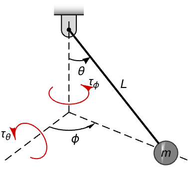
ℒ = (1/2) m L^2(Derivative[1][θ][t]^2 + Sin[θ[t]]^2 Derivative[1][ϕ][t]^2) + m g L Cos[θ[t]];eqns = Table[Subscript[∂, t]D[ℒ, q'[t]] - D[ℒ, q[t]] == Subscript[τ, q][t], {q, {θ, ϕ}}]该方程是仿射的并在 AffineStateSpaceModel 中精确表示:
AffineStateSpaceModel[eqns, {ϕ[t], θ[t]}, {Subscript[τ, θ][t], Subscript[τ, ϕ][t]}, {ϕ[t], θ[t]}, t]根据其哈密顿量
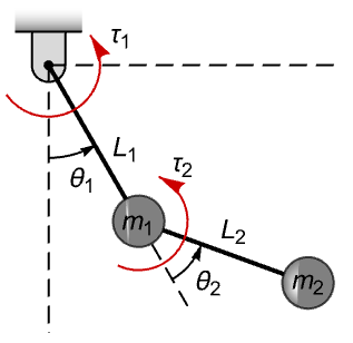
模拟双摆,其中
是广义坐标,
是广义动量,
是其拉格朗日量:
ℋ = (-2 g Cos[Subscript[θ, 1][t]] Subsuperscript[L, 1, 3] Subsuperscript[L, 2, 2] Subscript[m, 2] (Subscript[m, 1] + Subscript[m, 2]) (Subscript[m, 1] + Sin[Subscript[θ, 2][t]]^2 Subscript[m, 2]) + Subsuperscript[L, 2, 2] Subscript[m, 2] (Subscript[p, 1][t] - Subscript[p, 2][t])^2 - 2 Cos[Subscript[θ, 2][t]] Subscript[L, 1] Subscript[L, 2] Subscript[m, 2] (Subscript[p, 1][t] - Subscript[p, 2][t]) Subscript[p, 2][t] + Subsuperscript[L, 1, 2] (-2 g Cos[Subscript[θ, 1][t] + Subscript[θ, 2][t]] Subsuperscript[L, 2, 3] Subsuperscript[m, 2, 2] (Subscript[m, 1] + Sin[Subscript[θ, 2][t]]^2 Subscript[m, 2]) + (Subscript[m, 1] + Subscript[m, 2]) Subscript[p, 2][t]^2)) / (2 Subsuperscript[L, 1, 2] Subsuperscript[L, 2, 2] Subscript[m, 2] (Subscript[m, 1] + Sin[Subscript[θ, 2][t]]^2 Subscript[m, 2]));eqns1 = Table[D[Subscript[θ, i][t], t] == D[ℋ, Subscript[p, i][t]], {i, 2}];eqns2 = Table[Subscript[τ, i][t] - Subscript[p, i]'[t] == D[ℋ, Subscript[θ, i][t]], {i, 2}];pars = {Subscript[L, 1] -> 1, Subscript[L, 2] -> 1, Subscript[m, 1] -> 1, Subscript[m, 2] -> 1, g -> 9.8};AffineStateSpaceModel[Join[eqns1, eqns2], {Subscript[θ, 1][t], Subscript[θ, 2][t], Subscript[p, 1][t], Subscript[p, 2][t]}, {Subscript[τ, 1][t], Subscript[τ, 2][t]}, {Subscript[θ, 1][t], Subscript[θ, 2][t]}, t] /. pars//Simplify
pars = {l -> 1, m -> 0.2, M -> 0.3, g -> 9.8};eqns = {(M + m)x''[t] + m l Sin[θ[t]] θ'[t]^2 - m l Cos[θ[t]] θ''[t] == F[t], l θ''[t] - x''[t] Cos[θ[t]] - g Sin[θ[t]] == 0} /. pars;pend = AffineStateSpaceModel[eqns, {θ[t], x[t]}, {{F[t], 0}}, {θ[t], x[t]}, t]k = StateFeedbackGains[StateSpaceModel[pend], {-2, -3, -4, -5}]res = OutputResponse[{SystemsModelStateFeedbackConnect[pend, k], {40°, 0, 0, 0}}, 0, {t, 0, 4}];Plot[res, {t, 0, 4}, PlotRange -> All]模拟在梁上平衡的球. 求是否能仅从梁的角度
观察到所有的内部状态:
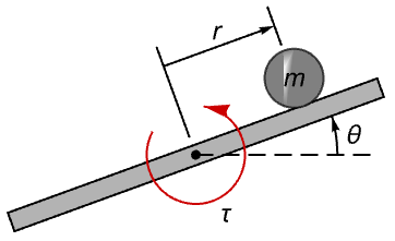
eqns = {r''[t] + g Sin[θ[t]] - r[t] θ'[t]^2 == 0, (m r[t]^2 + J)θ''[t] + 2 m r[t]r'[t]θ'[t] + m g r[t] Cos[θ[t]] == τ[t]};AffineStateSpaceModel[eqns, {r[t], θ[t]}, τ[t], {θ[t]}, t]ObservableModelQ[%]模拟汽车的动力学装置,其中控制输入为驱动速度和转向角速率. 说明该汽车可以通过控制输入的组合来对侧向运动进行控制:
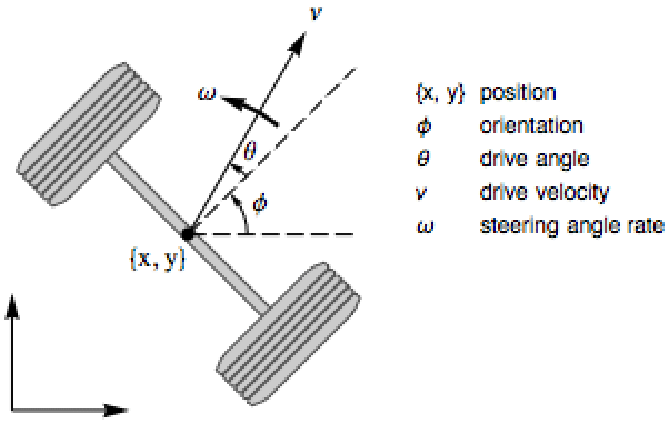
a = {0, 0, 0, 0};
b = {{Cos[θ + ϕ], 0}, {Sin[θ + ϕ], 0}, {Sin[θ], 0}, {0, 1}};car = AffineStateSpaceModel[{a, b, {x, y}}, {x, y, ϕ, θ}]AffineStateSpaceModel 表明汽车在各个方向都是可控的:
ControllableModelQ[car]ControllableModelQ[StateSpaceModel[car]]inp = {Piecewise[{{1, 0 <= t <= 1}, {0, Inequality[1, Less, t, LessEqual, 2]},
{-1, Inequality[2, Less, t, LessEqual, 3]}}, 0], Piecewise[{{0, 0 <= t <= 1}, {1, Inequality[1, Less, t, LessEqual, 2]},
{0, Inequality[2, Less, t, LessEqual, 3]}, {-1, Inequality[3, Less, t, LessEqual, 4]}}, 0] };{Subscript[x, r], Subscript[y, r], Subscript[ϕ, r], Subscript[θ, r]} = StateResponse[car, inp, {t, 0, 5}];axle = With[{x = 0.3, y = -0.3, d1 = 0.15, d2 = 0.025, d3 = 0.04, d4 = 0.6}, Polygon[{{x, y}, {x - d1, y}, {x - d1, y - d2}, {x + d1 + d3, y - d2}, {x + d1 + d3, y}, {x + d3, y}, {x + d3, y + d4}, {x + d1 + d3, y + d4}, {x + d1 + d3, y + d2 + d4}, {x - d1, y + d2 + d4}, {x - d1, y + d4}, {x, y + d4}}]];Animate[
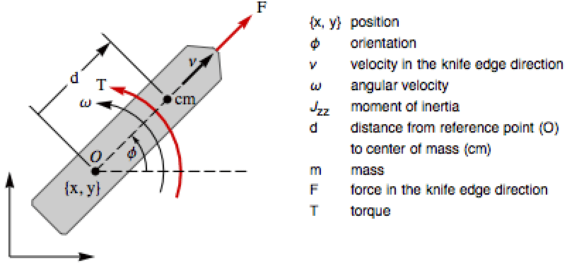
Evaluate[tfun = {RotationMatrix[Subscript[ϕ, r]], {Subscript[x, r], Subscript[y, r]}};Graphics[{Rotate[GeometricTransformation[axle, tfun], Subscript[θ, r]]}, PlotRange -> {{0, 1.75}, {-1.25, 0.5}}]], {t, 0, 5}, SaveDefinitions -> True, AnimationRunning -> False, AnimationRate -> 0.25]雪橇在水平面上的可控性,其中驱动力
和扭矩
为输入: »
a = {ω, Cos[ϕ] v, Sin[ϕ] v, -(d m ω v/d^2 m + Subscript[J, zz]), d ω^2};
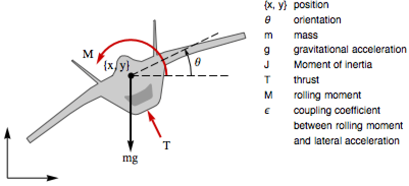
b = {{0, 0}, {0, 0}, {0, 0}, {(1/d^2 m + Subscript[J, zz]), 0}, {0, (1/m)}};sl = AffineStateSpaceModel[{a, b}, {ϕ, x, y, ω, v}]ControllableModelQ[StateSpaceModel@sl]Table[ControllableModelQ[SystemsModelExtract[sl, i]], {i, {1, 2}}]计算平面垂直起降(PVTOL)飞机的零动态: »
AffineStateSpaceModel[{m x''[t] == -Sin[θ[t]]T[t] + ϵ Cos[θ[t]] M[t], m y''[t] == Cos[θ[t]] T[t] + ϵ Sin[θ[t]] M[t] - m g, J θ''[t] == M[t]}, {x[t], y[t], θ[t]}, {T[t], M[t]}, {x[t], y[t]}, t]FeedbackLinearize[%, {{Subscript[z, 1], Subscript[z, 2], Subscript[z, 3], Subscript[z, 4], Subscript[z, 5], Subscript[z, 6]}}, "ZeroDynamicsSystem"]Eigenvalues[First[Normal[StateSpaceModel[%]]]]asys = AffineStateSpaceModel[{{0, 0, 0}, {{1, 0}, {0, 1}, {-Subscript[x, 2], Subscript[x, 1]}}}, {Subscript[x, 1], Subscript[x, 2], Subscript[x, 3]}]ControllableModelQ /@ {asys, StateSpaceModel[asys]}Electrical Systems (4)
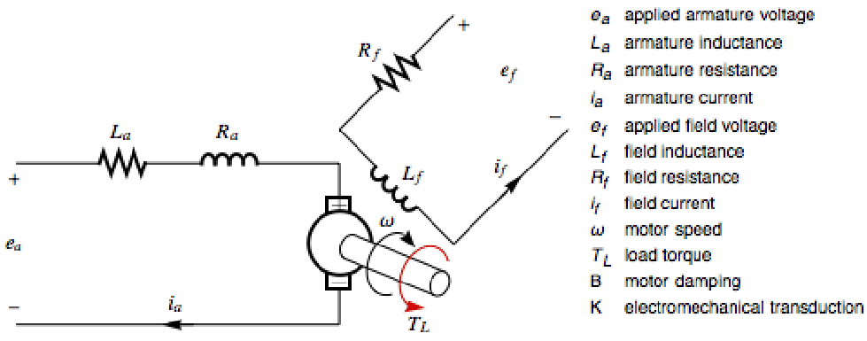
模拟一个他激式直流电动机,用电枢电压、励磁电压和负载转矩作为输入,并查看在线性近似磁极上阻尼的影响: »
aa = {(-B ω + K Subscript[i, a] Subscript[i, f]/J), (-K ω Subscript[i, f] - Subscript[i, a] Subscript[R, a]/Subscript[L, a]), -(Subscript[i, f] Subscript[R, f]/Subscript[L, f])};
bb = {{0, 0, -(1/J)}, {(1/Subscript[L, a]), 0, 0}, {0, (1/Subscript[L, f]), 0}};
cc = {ω};
xx = {ω -> 50, Subscript[i, a] -> 33.49727, Subscript[i, f] -> 1.25383};
uu = {Subscript[e, a] -> 283.65, Subscript[e, f] -> 75.23, Subscript[T, L] -> 10};asys = AffineStateSpaceModel[{aa, bb, cc}, xx, uu]pars = {K -> 0.25, J -> 0.15, Subscript[L, a] -> 2, Subscript[R, a] -> 8, Subscript[L, f] -> 8, Subscript[R, f] -> 60};tfm = TransferFunctionModel[asys /. pars]//SimplifyFirst@TransferFunctionZeros[tfm]//QuietRootLocusPlot[SystemsModelExtract[tfm, 1], {B, 0, 1}, FeedbackType -> None, AspectRatio -> 1, PlotRange -> All]模拟在 d-q (直-交)旋转坐标系中的感应电动机,并用它来获得一个相坐标作为输出的模型: »
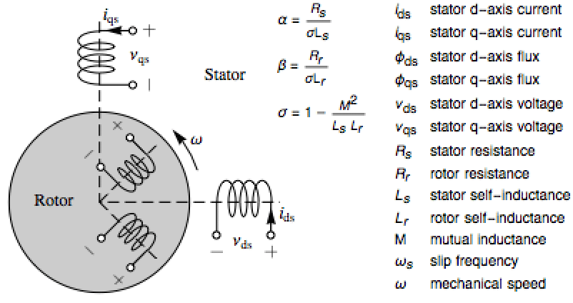
a = {-(α + β)Subscript[i, ds] + (β/Subscript[L, s])Subscript[ϕ, ds] + (ω/σ Subscript[L, s])Subscript[ϕ, qs], -(α + β)Subscript[i, qs] - (ω/σ Subscript[L, s])Subscript[ϕ, ds] + (β/Subscript[L, s])Subscript[ϕ, qs], -α σ Subscript[L, s]Subscript[i, ds] + ω Subscript[ϕ, qs], -α σ Subscript[L, s]Subscript[i, qs] - ω Subscript[ϕ, ds]};
b = {{(1/σ Subscript[L, s]), 0, Subscript[i, qs]}, {0, (1/σ Subscript[L, s]), -Subscript[i, ds]}, {1, 0, Subscript[ϕ, qs]}, {0, 1, -Subscript[ϕ, ds]}};motor = AffineStateSpaceModel[{a, b}, {Subscript[i, ds], Subscript[i, qs], Subscript[ϕ, ds], Subscript[ϕ, qs]}]trans = Inverse[{{Cos[Subscript[n, r] θ], Sin[Subscript[n, r] θ]}, {-Sin[Subscript[n, r] θ], Cos[Subscript[n, r] θ]}}]//Simplify;
TransferFunctionModel[ArrayFlatten[{{trans, 0}, {0, trans}}]]SystemsModelSeriesConnect[motor, %]使用运动学方程(它表示广义坐标和准速度之间的关系)和动态方程(通过庞加莱方程得到),组合三相同步电动机的模型. 输入是负载转矩
、布朗德尔电压
和绕组电压
: »
u = {Subscript[T, L][t], Subscript[v, d][t], Subscript[v, q][t], Subscript[v, o][t], Subscript[v, f][t]}qq = {θ[t], Subscript[q, 1][t], Subscript[q, 2][t], Subscript[q, 3][t], Subscript[q, f][t]}p = {ω[t], Subscript[i, d][t], Subscript[i, q][t], Subscript[i, 0][t], Subscript[i, f][t]}V = {{1, 0, 0, 0, 0}, {0, Sqrt[(2/3)] Cos[θ[t]], -Sqrt[(2/3)] Sin[(π/6) - θ[t]], -Sqrt[(2/3)] Sin[(π/6) + θ[t]], 0}, {0, Sqrt[(2/3)] Sin[θ[t]], -Sqrt[(2/3)] Cos[(π/6) - θ[t]], Sqrt[(2/3)] Cos[(π/6) + θ[t]], 0}, {0, (1/Sqrt[3]), (1/Sqrt[3]), (1/Sqrt[3]), 0}, {0, 0, 0, 0, 1}};c[i_, j_, k_] := V[[i]].(D[V[[k]], {qq}].V[[j]] - D[V[[j]], {qq}].V[[k]])ℒ = (1/2)p.(| | | | | |
| - | ------------- | ------- | --------- | ------------- |
| J | 0 | 0 | 0 | 0 |
| 0 | L1 + L3 | 0 | 0 | Sqrt[(3/2)]L5 |
| 0 | 0 | L1 + L3 | 0 | 0 |
| 0 | 0 | 0 | L1 - 2 L3 | 0 |
| 0 | Sqrt[(3/2)]L5 | 0 | 0 | L4 |).p//Simplify𝒟 = (1/2)p.DiagonalMatrix[{0, r, r, r, Subscript[r, f]}].p + {-Subscript[T, L][t], Subscript[v, d][t], Subscript[v, q][t], Subscript[v, o][t], Subscript[v, f][t]}.p;𝒬 = D[𝒟, {p}]peqns = Thread[Table[D[D[ℒ, p[[kk]]], t] - Underoverscript[∑, ii = 1, 5]Underoverscript[∑, jj = 1, 5]c[ii, jj, kk]D[ℒ, p[[ii]]]p[[jj]], {kk, Range[5]}] == 𝒬]//FullSimplifyAffineStateSpaceModel[Join[Thread[D[qq, t] == V.p], peqns], Join[qq, p], u, {}, t] /. Subscript[L, _] -> 1//FullSimplify对不同的非线性特性模拟蔡氏电路:»
pars = {Subscript[𝒞, 1] -> (1/9), Subscript[𝒞, 2] -> 1, ℒ -> (1/7), ℛ -> (1/0.7)};chua[g_, v_] := AffineStateSpaceModel[{{(1/Subscript[𝒞, 1])((1/ℛ)(Subscript[𝒱, 2] - v) - g), (1/Subscript[𝒞, 2])((1/ℛ)(v - Subscript[𝒱, 2]) - 𝒾), (1/ℒ)Subscript[𝒱, 2]}, {{-1}, {0}, {0}}, {v, Subscript[𝒱, 2]}}, {v -> -0.2, Subscript[𝒱, 2] -> 0, 𝒾 -> 1}] /. parschua[g[Subscript[𝒱, 1]], Subscript[𝒱, 1]]resp[g_, v_] := (or = OutputResponse[chua[g, v], 0, {t, 0, 90}];
Tooltip[ParametricPlot[or, {t, 0, 90}, PlotRange -> All], Plot[g, {v, -5, 5}]]
)resp[Piecewise[{{0.9 - 0.55*(1 + v), v < -1}, {-0.9*v, -1 <= v <= 1}, {-0.9 - 0.15*(-1 + v), v > 1}}, 0], v]resp[Piecewise[{{0.7 - 0.15*(1 + v), v < -1}, {-0.7*v, -1 <= v <= 1}, {-0.7 - 0.15*(-1 + v), v > 1}}, 0], v]resp[-0.52v + 0.0006 v^3, v]resp[-0.5 v, v]Chemical Systems (5)
比较仿射模型和线性模型对连续发酵反应的模拟: »
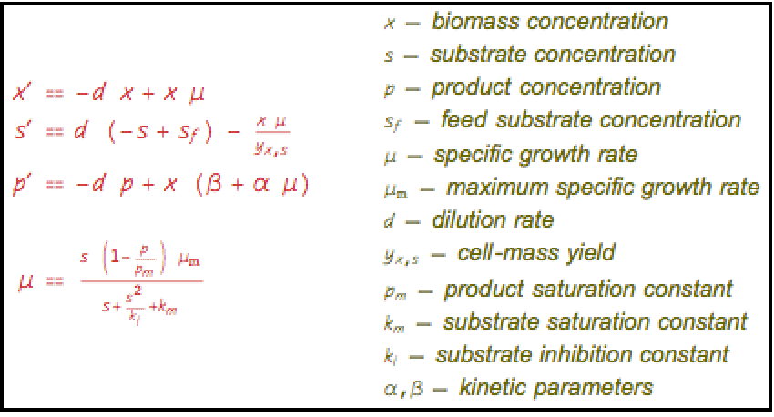
a = With[{μ = Subscript[μ, 𝓂](1 - 𝓅 / Subscript[𝓅, 𝓂])𝓈 / (Subscript[𝓀, 𝓂] + 𝓈 + 𝓈^2 / Subscript[𝓀, 𝒾])}, {-𝒹 𝓍 + μ 𝓍, -𝒹 𝓈 - μ 𝓍 / Subscript[𝓎, 𝓍, 𝓈], -𝒹 𝓅 + (α μ + β) 𝓍}];
b = {{0}, {𝒹}, {0}};
c = {𝒹 𝓅};asys = AffineStateSpaceModel[{a, b, c}, {𝓍, 𝓈, 𝓅}]lsys = StateSpaceModel[asys]pars = {Subscript[μ, 𝓂] -> 0.48, 𝒹 -> 0.15, Subscript[𝓎, 𝓍, 𝓈] -> 0.4, Subscript[𝓅, 𝓂] -> 50, Subscript[𝓀, 𝓂] -> 1.2, Subscript[𝓀, 𝒾] -> 22, α -> 2.2, β -> 0.2};Table[OutputResponse[{sys, {0.1, 0.5, 0}}, 0, {t, 0, 30}], {sys, {asys, lsys} /. pars}];Plot[%, {t, 0, 30}, PlotLegends -> {"Affine response", "Linear response"}]对于使用频率技术在非等温连续搅拌釜式反应器(CSTR)中的反应,比较仿射模型和线性模型: »

aa = With[{c = (1 - Subscript[x, 1])Exp[Subscript[x, 2] / (1 + Subscript[x, 2] / γ)]}, {-Subscript[x, 1] + Subscript[d, a] c, -Subscript[x, 2] + b Subscript[d, a]c - β Subscript[x, 2]}];
bb = {{0}, {β}};
cc = {Subscript[x, 2]};pars = {β -> 1, Subscript[d, a] -> 1, b -> 1, γ -> 1};asys = AffineStateSpaceModel[{aa, bb, cc}, {Subscript[x, 1], Subscript[x, 2]}] /. pars通过关于原点的泰勒线性化,得到它的 TransferFunctionModel:
tfm = TransferFunctionModel[asys]BodePlot 给出线性系统的频率响应:
sfreq = Log10[1];BodePlot[tfm, Epilog -> {Line[{{sfreq, -40}, {sfreq, 0}}], Line[{{sfreq, -90}, {sfreq, 0}}]}]{Power[10, -4.1 / 20], 30 °}//Nlres = OutputResponse[tfm, Sin[t], {t, 0, 50}];
nlres = OutputResponse[asys, Sin[t], {t, 0, 50}];下图表明,与线性化系统的预测相比,仿射系统的衰减较小,但相位滞后较大:
Plot[{Sin[t], lres, nlres}, {t, 0, 12}, PlotLegends -> {"Input", "Response of linear system", "Response of affine system"}]在等温 CSTR 中,得到反应的零动态
: »
aa = {1 - Subscript[𝓍, 𝒜] - Subscript[𝒟𝒶, 𝒶1]Subscript[𝓍, 𝒜] + Subscript[𝒟𝒶, 𝒶2]Subsuperscript[𝓍, ℬ, 2], -Subscript[𝓍, ℬ] + Subscript[𝒟𝒶, 𝒶1]Subscript[𝓍, 𝒜] - Subscript[𝒟𝒶, 𝒶2]Subsuperscript[𝓍, ℬ, 2] - Subscript[𝒟𝒶, 𝒶3]Subsuperscript[𝓍, 𝒞, 2], -Subscript[𝓍, 𝒞] + Subscript[𝒟𝒶, 𝒶3]Subsuperscript[𝓍, ℬ, 2]};
bb = {{0}, {1}, {0}};
cc = {Subscript[𝓍, 𝒞]};asys = AffineStateSpaceModel[{aa, bb, cc}, {Subscript[𝓍, 𝒜], Subscript[𝓍, ℬ], Subscript[𝓍, 𝒞]}]SystemsModelVectorRelativeOrders[asys]FeedbackLinearize[asys, Automatic, "ZeroDynamicsSystem"]Eigenvalues@First@Normal@StateSpaceModel@%使用精确线性化设计一个调节器,调节环戊烯醇合成过程
,
中
和
的浓度,其中
和
是环戊二醇(cylopentandiol)和二环戊二烯(dicyclopentadien): »
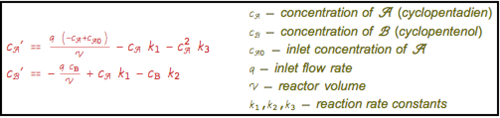
pars = {𝓊 -> 0.2, Subscript[𝓀, 1] -> 0.05, Subscript[𝓀, 2] -> 0.01, Subscript[𝓀, 3] -> 0.025, Subscript[𝒸, 𝒜0] -> 0.3};aa = {-Subscript[𝓀, 1] Subscript[𝒸, 𝒜] - Subscript[𝓀, 3]Subsuperscript[𝒸, 𝒜, 2], Subscript[𝓀, 1]Subscript[𝒸, 𝒜] - Subscript[𝓀, 2]Subscript[𝒸, ℬ]};
bb = {{(Subscript[𝒸, 𝒜0] - Subscript[𝒸, 𝒜])}, {-Subscript[𝒸, ℬ]}};
cc = {Subscript[𝒸, ℬ]};Join[Thread[(aa + bb.{𝓊} /. pars) == 0], {Subscript[𝒸, 𝒜] > 0, Subscript[𝒸, ℬ] > 0}];sols = NSolve[%, {Subscript[𝒸, 𝒜], Subscript[𝒸, ℬ]}]asys = AffineStateSpaceModel[{aa, bb, cc} /. pars, sols[[1]], {𝓊 -> 0.2}]ℱ = FeedbackLinearize[asys, {{Subscript[z, 1], Subscript[z, 2]}, v}]Eigenvalues[First@Normal@StateSpaceModel@ℱ["ResidualSystem"]]κ = StateFeedbackGains[ℱ["LinearSystem"], {-5}]csys = ℱ[{"ClosedLoopSystem", κ}]OutputResponse[{csys, {0.09, 0.1}}, 0, {t, 0, 5}];
p1 = Plot[%, {t, 0, 5}, PlotRange -> {{0, 1.5}, All}]OutputResponse[{asys, {0.09, 0.1}}, 0, {t, 0, 5}];
Show[p1, Plot[%, {t, 0, 5}, PlotRange -> All, PlotStyle -> Dashed]]气体保护电弧焊过程可以用仿射系统进行模拟. 设计一个可以保持指定弧长的反馈律: »
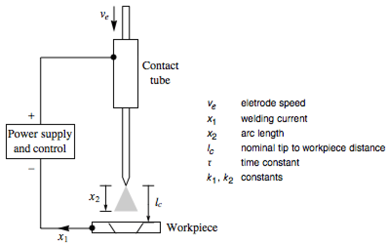
pars = {Subscript[k, 1] -> (3/10000), Subscript[k, 2] -> (7/10000), Subscript[v, e] -> 0.3, τ -> (7/100000)};asys = AffineStateSpaceModel[{{(-τ^(-1))*Subscript[x, 1][t],
-Subscript[v, e] + Subscript[k, 1]*
Subscript[x, 1][t] + Subscript[k, 2]*
Subscript[x, 1][t]^2*(Subscript[l, c] -
Subscript[x, 2][t])}, {{τ^(-1)}, {0}},
{Subscript[x, 2][t]}, {{0}}},
{Subscript[x, 1][t], Subscript[x, 2][t]},
Automatic, {Automatic}, t, SamplingPeriod -> None] /. pars;计算反馈律,使用 AsymptoticOutputTracker 保持弧长为1厘米:
fb = AsymptoticOutputTracker[asys, 0.01, {-15, -20}]//SimplifyRandomFunction[WhiteNoiseProcess[0.001], {0, 10}]["Paths"][[1]];
Subscript[l, c] = Interpolation[{#[[1]], #[[2]] + 0.02}& /@ %, t];Plot[Subscript[l, c], {t, 0, 10}]csys = SystemsModelStateFeedbackConnect[asys, fb];Plot[OutputResponse[{csys, {200, 0.01}}, {0}, {t, 0, 10}]//Evaluate, {t, 0, 10}, PlotRange -> All, AxesOrigin -> {0, 0}]属性和关系 (4)
通过线性化状态和输入,AffineStateSpaceModel 转换为 StateSpaceModel:
StateSpaceModel[AffineStateSpaceModel[{{Subscript[x, 2], Subscript[x, 1] +
Subscript[x, 2]^2}, {{0}, {1 + Subscript[x, 2]}},
{Subscript[x, 1]}, {{0}}}, {{Subscript[x, 1], 0},
{Subscript[x, 2], 0}}, {{u, 0}}, {Automatic}, Automatic,
SamplingPeriod -> None]]AffineStateSpaceModel[%]通过线性化输入,NonlinearStateSpaceModel 转换为 AffineStateSpaceModel:
AffineStateSpaceModel[NonlinearStateSpaceModel[{{Subscript[x, 2],
u^2 + Subscript[x, 1] + Subscript[x, 2]^2 +
u*(1 + Subscript[x, 2])}, {Subscript[x, 1]}},
{{Subscript[x, 1], 0}, {Subscript[x, 2], 0}}, {{u, 0}},
{Automatic}, Automatic, SamplingPeriod -> None]]NonlinearStateSpaceModel[%]通过状态和输入线性化,转换为 TransferFunctionModel:
TransferFunctionModel[AffineStateSpaceModel[{{Subscript[x, 2], Subscript[x, 1] +
Subscript[x, 2]^2}, {{0}, {1 + Subscript[x, 2]}},
{Subscript[x, 1]}, {{0}}}, {{Subscript[x, 1], 0},
{Subscript[x, 2], 0}}, {{u, 0}}, {Automatic}, Automatic,
SamplingPeriod -> None], s]AffineStateSpaceModel[%]StateSpaceTransform 可能生成 NonlinearStateSpaceModel:
sys = AffineStateSpaceModel[{{-Subscript[x, 2], Subscript[x, 1]}, {{0}, {u}}}, {Subscript[x, 1], Subscript[x, 2]}, u]StateSpaceTransform[sys, {{1, 0}, {0, 1}}]可能存在的问题 (1)
a = {Subscript[x, 1] Exp[Subscript[x, 3]], -Subscript[x, 1], Subscript[x, 1]Subscript[x, 2]};
b1 = {0, Subscript[x, 2], 1};b2 = {-1, 0, 1};AffineStateSpaceModel[{a, {b1, b2}, Subscript[x, 1]}, {Subscript[x, 1], Subscript[x, 2], Subscript[x, 3]}]使用 Transpose 把它们按列排列:
AffineStateSpaceModel[{a, Transpose[{b1, b2}], Subscript[x, 1]}, {Subscript[x, 1], Subscript[x, 2], Subscript[x, 3]}]文本
Wolfram Research (2014),AffineStateSpaceModel,Wolfram 语言函数,https://reference.wolfram.com/language/ref/AffineStateSpaceModel.html.
CMS
Wolfram 语言. 2014. "AffineStateSpaceModel." Wolfram 语言与系统参考资料中心. Wolfram Research. https://reference.wolfram.com/language/ref/AffineStateSpaceModel.html.
APA
Wolfram 语言. (2014). AffineStateSpaceModel. Wolfram 语言与系统参考资料中心. 追溯自 https://reference.wolfram.com/language/ref/AffineStateSpaceModel.html 年
BibTeX
@misc{reference.wolfram_2026_affinestatespacemodel, author="Wolfram Research", title="{AffineStateSpaceModel}", year="2014", howpublished="\url{https://reference.wolfram.com/language/ref/AffineStateSpaceModel.html}", note=[Accessed: 19-August-2026]}
BibLaTeX
@online{reference.wolfram_2026_affinestatespacemodel, organization={Wolfram Research}, title={AffineStateSpaceModel}, year={2014}, url={https://reference.wolfram.com/language/ref/AffineStateSpaceModel.html}, note=[Accessed: 19-August-2026]}