

BeckmannDistribution[μ1,μ2,σ1,σ2]
平均が μ1,μ2,標準偏差が σ1,σ2のBeckmann分布を表す.
BeckmannDistribution[μ1,μ2,σ1,σ2,ρ]
平均が μ1,μ2,標準偏差が σ1,σ2,相関が ρ のBeckmann分布を表す.
BeckmannDistribution
BeckmannDistribution[μ1,μ2,σ1,σ2]
平均が μ1,μ2,標準偏差が σ1,σ2のBeckmann分布を表す.
BeckmannDistribution[μ1,μ2,σ1,σ2,ρ]
平均が μ1,μ2,標準偏差が σ1,σ2,相関が ρ のBeckmann分布を表す.
詳細
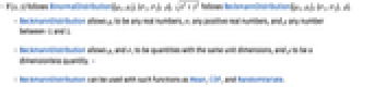
- {x,y}がBinormalDistribution[{μ1,μ2},{σ1,σ2}, ρ]に従うなら,

はBeckmannDistribution[{μ1,μ2},{σ1,σ2}, ρ]に従う. - BeckmannDistributionでは,μiは任意の実数でよく,σiは任意の正の実数でよく,ρ は-1から1までの任意の数でよい.
- BeckmannDistributionでは,μiと σiは単位次元が等しい数量でよく,ρ は無次元量でよい. »
- BeckmannDistributionは,Mean,CDF,RandomVariate等の関数とともに使うことができる.
予備知識
- BeckmannDistribution[μ1,μ2,σ1,σ2,ρ]は,区間
上で定義され,数 μ1,μ2,σ1,σ2,ρ によってパラメータ化される連続確率分布を表す.ここで,μ1および μ2は任意の実数,σ1および σ2は正の実数,ρ は

を満足する実数である.Beckmann分布の確率密度関数(PDF)の全体的な形はその引数に依存する.例えば,Beckmann分布のPDFは,常に単峰型であるが,峰の周囲(くぼんだ部分)のPDFの形はその引数に依存する.一般に,σiの値が高くなる程,峰の周囲のPDFの「険しさ」が増し,値が低くなるにつれ分布は峰の識別しやすさが減ずるように「広がる」.パラメータ μiを変化させることで,PDFの高さと水平位置の両方を変えることができ,ρ を変えることで高さと全体的な凹面に影響が出る.4引数形のBeckmannDistribution[μ1,μ2,σ1,σ2]はBeckmannDistribution[μ1,μ2,σ1,σ2,0]に等しく,無相関Beckmann分布と呼ばれることがある. - BeckmannDistribution[μ1,μ2,σ1,σ2,ρ]は,ペア
の各要素がBinormalDistribution[{μ1,μ2},{σ1,σ2}, ρ]に従って分布しているときに,

が従う分布として定義される.結果として,正規分布に従い相関している要素を持つ二次元ベクトルのノルムは Beckmann分布に従う.Beckmann分布は,科学的可視化,特に三次元コンピュータグラフィックスの陰影付けと鏡面ハイライトに根本的な役割を果たし,フェージングチャネル理論のフェージング振幅のモデル化に使われる. - RandomVariateを使ってBeckmann分布から,1つあるいは複数の機械精度あるいは任意精度(後者はWorkingPrecisionオプションを介す)の擬似乱数変量を得ることができる.Distributed[x,BeckmannDistribution[μ1,μ2,σ1,σ2,ρ]](より簡略すると xBeckmannDistribution[μ1,μ2,σ1,σ2,ρ])を使って,確率変数 x がBeckmann分布に従って分布していると宣言することができる.このような宣言は,Probability,NProbability,Expectation,NExpectation等の関数で使うことができる.
- 確率密度関数および累積分布関数は,PDF[BeckmannDistribution[μ1,μ2,σ1,σ2,ρ],x]およびCDF[BeckmannDistribution[μ1,μ2,σ1,σ2,ρ],x]を使って得られることがある.平均,中央値,分散,原点の周りのモーメント,中心モーメントは,それぞれMean,Median,Variance,Moment,CentralMomentを使って計算することができる.
- DistributionFitTestを使って,与えられたデータ集合がBeckmann分布と一致するかどうかを検定することが,EstimatedDistributionを使って与えられたデータからBeckmannパラメトリック分布を推定することが,FindDistributionParametersを使ってデータをBeckmann分布にフィットすることができる.ProbabilityPlotを使って記号Beckmann分布のCDFに対する与えられたデータのCDFのプロットを生成することが,QuantilePlotを使って記号Beckmann分布の変位値に対する与えられたデータの変位値のプロットを生成することができる.
- TransformedDistributionを使って変換されたBeckmann分布を表すことが,CensoredDistributionを使って上限値と下限値の間で切り取られた値の分布を表すことが,TruncatedDistributionを使って上限値と下限値の間で切断された値の分布を表すことができる.CopulaDistributionを使ってBeckmann分布を含む高次元分布を構築することが,ProductDistributionを使ってBeckmann分布を含む独立成分分布の結合分布を計算することができる.
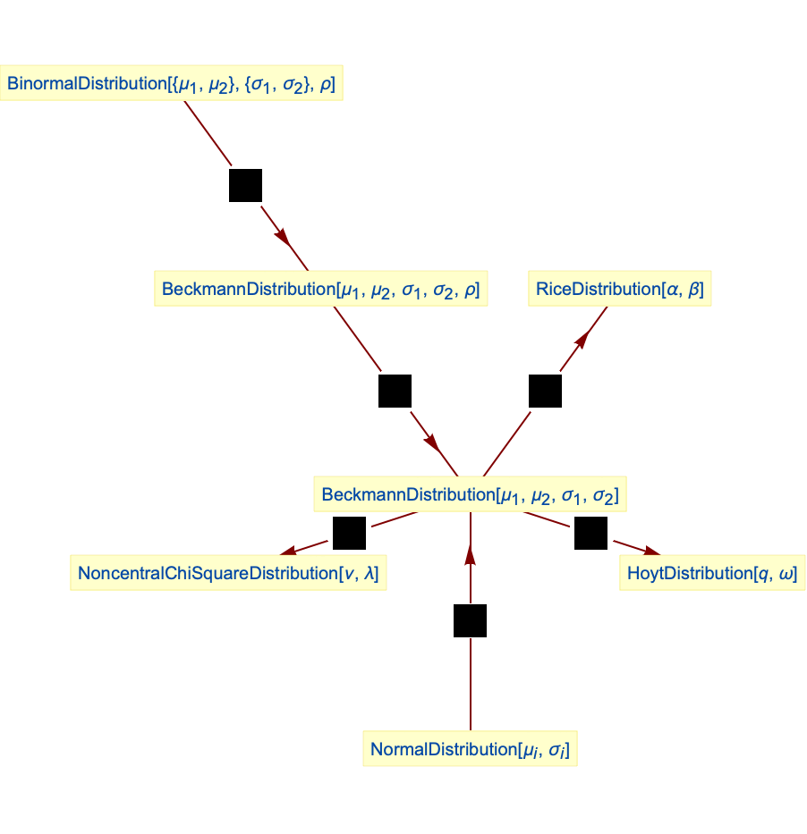
- BeckmannDistributionは他の数多くの分布と密接な関係がある.例えばBeckmannDistributionはNormalDistributionおよびBinormalDistributionの両方の変換として実現することができ,それ自身を変換してNoncentralChiSquareDistributionを実現することができる.さらに,HoytDistributionおよびRiceDistributionはどちらもBeckmannDistributionの特殊ケースである.
例題
すべて開く すべて閉じる例 (2)
Plot[Table[PDF[BeckmannDistribution[1, -2, 2, σ2], x], {σ2, {1 / 2, 1, 2}}]//Evaluate, {x, 0, 8}, Filling -> Axis]Plot[Table[PDF[BeckmannDistribution[1, μ2, 2, 3], x], {μ2, {-4, 1, 3}}]//Evaluate, {x, 0, 10}, Filling -> Axis]Plot[Table[PDF[BeckmannDistribution[1, -2, 2, 3, ρ], x], {ρ, {-.9, 0, .9}}]//Evaluate, {x, 0, 8}, Filling -> Axis]Plot[Table[CDF[BeckmannDistribution[1, -2, 2, σ2], x], {σ2, {1 / 2, 1, 2}}]//Evaluate, {x, 0, 8}, Filling -> Axis]Plot[Table[CDF[BeckmannDistribution[1, μ2, 2, 3], x], {μ2, {-4, 1, 3}}]//Evaluate, {x, 0, 10}, Filling -> Axis]Plot[Table[CDF[BeckmannDistribution[1, -2, 2, 3, ρ], x], {ρ, {-.9, 0, .9}}]//Evaluate, {x, 0, 8}, Filling -> Axis]スコープ (5)
data = RandomVariate[BeckmannDistribution[-1, 2, .5, 2], 10 ^ 4];Show[Histogram[data, 20, "PDF"], Plot[PDF[BeckmannDistribution[-1, 2, .5, 2], x], {x, 0, 8}, PlotStyle -> Thick]]sample = RandomVariate[BeckmannDistribution[3, 2, .5, .3], 10 ^ 2];edist = EstimatedDistribution[sample, BeckmannDistribution[3, 2, σ1, σ2]]サンプルの密度ヒストグラムを推定分布の確率密度関数と比較する:
Show[Histogram[sample, Automatic, "PDF"], Plot[PDF[edist, x], {x, 0, 5}, PlotStyle -> Thick]]Plot[Table[HazardFunction[BeckmannDistribution[1, -2, 2, σ2], x], {σ2, {1 / 2, 1, 2}}]//Evaluate, {x, 0, 6}, Filling -> Axis]Plot[Table[HazardFunction[BeckmannDistribution[1, μ2, 2, 3], x], {μ2, {-4, 1, 3}}]//Evaluate, {x, 0, 6}, Filling -> Axis]Plot[Table[HazardFunction[BeckmannDistribution[1, -2, 2, 3, ρ], x], {ρ, {-.9, 0, .9}}]//Evaluate, {x, 0, 6}, Filling -> Axis]Plot[Table[Quantile[BeckmannDistribution[1, -2, 2, σ2], q], {σ2, {1 / 2, 1, 2}}]//Evaluate, {q, .01, .99}, Filling -> Axis]Plot[Table[Quantile[BeckmannDistribution[1, μ2, 2, 3], q], {μ2, {-4, 1, 3}}]//Evaluate, {q, .01, .99}, Filling -> Axis]母数でQuantityを一貫して使うとQuantityDistributionが与えられる:
dist𝒟 = BeckmannDistribution[Quantity[182, "Centimeters"], Quantity[200, "Centimeters"], Quantity[10, "Centimeters"], Quantity[7, "Centimeters"], 0.34]Quartiles[dist𝒟]アプリケーション (2)
正規分布に従い相関性がある要素を持つ2Dベクトルの長さはBeckmann分布に従う:
𝒟 = Block[{μ1 = Quantity[3, "Centimeters"], μ2 = Quantity[1, "Centimeters"], σ1 = Quantity[0.5, "Centimeters"], σ2 = Quantity[0.1, "Centimeters"], ρ = 0.2}, BeckmannDistribution[μ1, μ2, σ1, σ2, ρ]];Plot[PDF[𝒟, Quantity[x, "Centimeters"]], {x, 0, 6}, Filling -> Axis, AxesLabel -> {"cm"}]Probability[x ≥ Quantity[3.5, "Centimeters"], x𝒟]Mean[𝒟]30のサンプルベクトルの考えられる長さのシミュレーションを行う:
ListPlot[{RandomVariate[𝒟, 30], {{0, Mean[𝒟]}, {30, Mean[𝒟]}}}, Joined -> {False, True}, Filling -> Axis, AxesLabel -> Automatic]フェージングチャネル理論では,BeckmannDistributionを使ってフェージング振幅モデル化が行われる.瞬間的な信号対ノイズ比の分布を求める.ただし,

,
は記号あたりのエネルギー,
はホワイトノイズのスペクトル密度である:
snd𝒟 = TransformedDistribution[ρ u ^ 2, uBeckmannDistribution[μ1, μ2, σ1, σ2]];Mean[snd𝒟]AF[dist_] := Variance[dist] / (Mean[dist]) ^ 2AF[snd𝒟]//FullSimplifyAF[snd𝒟] /. {μ1 -> 0, μ2 -> 0, σ1 -> 1, σ2 -> 1}AF[snd𝒟] /. {μ1 -> 0, μ2 -> 0, σ1 -> σ, σ2 -> σ}AF[snd𝒟] /. {μ1 -> α / Sqrt[2], μ2 -> α / Sqrt[2], σ1 -> β, σ2 -> β}//FullSimplifyAF[snd𝒟] /. {μ1 -> 0, μ2 -> 0, σ2 -> q σ1}//FullSimplify特性と関係 (8)
Beckmann分布は正の数でのスケーリングの下では閉じている:
TransformedDistribution[k u, uBeckmannDistribution[μ1, μ2, σ1, σ2]]TransformedDistribution[k u, uBeckmannDistribution[μ1, μ2, σ1, σ2, ρ]]
𝒟 = BeckmannDistribution[μ1, μ2, σ1, σ2, ρ];Block[{μ1 = -3, μ2 = 1, σ1 = 2, σ2 = 3, ρ = 0}, Show[Histogram[RandomVariate[𝒟, 10 ^ 4], 20, "PDF"], Plot[PDF[BeckmannDistribution[μ1, μ2, σ1, σ2], x], {x, 0, 12}, PlotStyle -> Thick]]]Beckmann分布はNoncentralChiSquareDistributionに関連している:
𝒟 = TransformedDistribution[x^2, xBeckmannDistribution[μ1, μ2, 1, 1]];Block[{μ1 = 3, μ2 = 4}, Show[Histogram[RandomVariate[𝒟, 10 ^ 4], 30, "PDF"], Plot[PDF[NoncentralChiSquareDistribution[2, μ1 ^ 2 + μ2 ^ 2], x], {x, 0, 60}, PlotStyle -> Thick]]]NormalDistributionに従う2要素のベクトルのノルムはBeckmann分布に従う:
𝒟 = TransformedDistribution[Norm[{u, v}], {uNormalDistribution[μ1, σ1], vNormalDistribution[μ2, σ2]}];Block[{μ1 = -2, μ2 = 3, σ1 = 0.5, σ2 = 1.5}, Show[Histogram[RandomVariate[𝒟, 10 ^ 4], 20, "PDF"], Plot[PDF[BeckmannDistribution[μ1, μ2, σ1, σ2], x], {x, 0, 10}, PlotStyle -> Thick]]]Beckmann分布はBinormalDistributionに関連している:
𝒟 = TransformedDistribution[Norm[{u, v}], {u, v}BinormalDistribution[{μ1, μ2}, {σ1, σ2}, ρ]];Block[{μ1 = 2, μ2 = 3, σ1 = 0.5, σ2 = 1.5, ρ = 0.7}, Show[Histogram[RandomVariate[𝒟, 10 ^ 3], 20, "PDF"], Plot[PDF[BeckmannDistribution[μ1, μ2, σ1, σ2, ρ], x], {x, 0, 10}, PlotStyle -> Thick]]]HoytDistributionはBeckmann分布から得ることができる:
𝒟 = BeckmannDistribution[0, 0, Sqrt[ω / (1 + q ^ 2)], q Sqrt[ω / (1 + q ^ 2)]];Block[{q = .8, ω = 6}, Show[Histogram[RandomVariate[𝒟, 10 ^ 4], 20, "PDF"], Plot[PDF[HoytDistribution[q, ω], x], {x, 0, 7}, PlotStyle -> Thick]]]RiceDistributionはBeckmann分布の特殊ケースである:
𝒟 = BeckmannDistribution[α / Sqrt[2], α / Sqrt[2], β, β];Block[{α = 2, β = .7}, Show[Histogram[RandomVariate[𝒟, 10 ^ 4], 20, "PDF"], Plot[PDF[RiceDistribution[α , β], x], {x, 0, 5}, PlotStyle -> Thick]]]おもしろい例題 (1)
累積分布関数の等高線を持つ σ2のさまざまな値についての確率密度関数:
dist = BeckmannDistribution[1, -2, 2, σ2];cdf = Function[{x, σ2}, Evaluate[CDF[dist, x]]];
ql = {0.025, 0.10, 0.25, 0.5, 0.75, 0.90, 0.975};
cl = Table[ColorData["Rainbow"][q], {q, Join[{0.0}, ql]}];Legended[Plot3D[PDF[dist, x], {x, 0, 8}, {σ2, 1, 3}, PlotTheme -> "Marketing", MeshFunctions -> {cdf}, Mesh -> {ql}, MeshStyle -> GrayLevel[0.8], PlotRange -> All, MeshShading -> cl, AxesLabel -> Automatic, BaseStyle -> Opacity[0.9], ImageSize -> 400], BarLegend["Rainbow", ql, LegendLabel -> "prob"]]関連するガイド
テキスト
Wolfram Research (2010), BeckmannDistribution, Wolfram言語関数, https://reference.wolfram.com/language/ref/BeckmannDistribution.html (2016年に更新).
CMS
Wolfram Language. 2010. "BeckmannDistribution." Wolfram Language & System Documentation Center. Wolfram Research. Last Modified 2016. https://reference.wolfram.com/language/ref/BeckmannDistribution.html.
APA
Wolfram Language. (2010). BeckmannDistribution. Wolfram Language & System Documentation Center. Retrieved from https://reference.wolfram.com/language/ref/BeckmannDistribution.html
BibTeX
@misc{reference.wolfram_2026_beckmanndistribution, author="Wolfram Research", title="{BeckmannDistribution}", year="2016", howpublished="\url{https://reference.wolfram.com/language/ref/BeckmannDistribution.html}", note=[Accessed: 17-August-2026]}
BibLaTeX
@online{reference.wolfram_2026_beckmanndistribution, organization={Wolfram Research}, title={BeckmannDistribution}, year={2016}, url={https://reference.wolfram.com/language/ref/BeckmannDistribution.html}, note=[Accessed: 17-August-2026]}