BinormalDistribution[{μ1,μ2},{σ1,σ2},ρ]
平均{μ1,μ2},共分散行列{{σ12,ρ σ1 σ2},{ρ σ1 σ2,σ22}}の二変量正規分布を表す.
BinormalDistribution[{σ1,σ2},ρ]
平均がゼロの二変量正規分布を表す.
平均がゼロで共分散行列が{{1,ρ },{ρ,1}}の二変量正規分布を表す.
BinormalDistribution
BinormalDistribution[{μ1,μ2},{σ1,σ2},ρ]
平均{μ1,μ2},共分散行列{{σ12,ρ σ1 σ2},{ρ σ1 σ2,σ22}}の二変量正規分布を表す.
BinormalDistribution[{σ1,σ2},ρ]
平均がゼロの二変量正規分布を表す.
平均がゼロで共分散行列が{{1,ρ },{ρ,1}}の二変量正規分布を表す.
詳細

- 二変量正規分布におけるベクトル
の確率密度は
に比例する. - BinormalDistributionでは,μiは任意の実数,σiは任意の正の実数,ρ は-1から1までの任意の数でよい.
- BinormalDistributionでは,μiと σiは成分ごとに単位次元が等しい数量でよく,ρ は無次元量でよい. »
- BinormalDistributionは,Mean,CDF,RandomVariate等の関数とともに使うことができる.
予備知識
- BinormalDistribution[{μ1,μ2},{σ1,σ2},ρ]は,最初と2番目の周辺分布(MarginalDistribution)のそれぞれがNormalDistributionである(変数
および
がx1NormalDistribution[μ1,σ1]およびx2NormalDistribution[μ2,σ2]をそれぞれ満足する)という特性を持つ,実数のペア上で定義された二変量(すなわち二変数)の統計分布を表す.二変量正規分布は,したがって,平均ベクトルと呼ばれる1組の実数ペア(μ1,μ2),標準偏差ベクトルと呼ばれる1組の正の実数のペア(σ1,σ2),
と
の相関として知られる
の1つの実数によってパラメータ化されている.ρ は,分布の随伴共分散行列
,つまり,
番目の項が変数
と
の間の共分散である2×2行列の定義に使われる. - 2引数形式のBinormalDistribution[{σ1,σ2},ρ]はBinormalDistribution[{0,0},{σ1,σ2},ρ]に等しいのに対し,1引数形式のBinormalDistribution[ρ]はBinormalDistribution[{0,0},{1,1},ρ]に等しく,標準二変量正規分布と呼ばれることがある.二変量正規分布に従う確率変数は,二変量正規変量と呼ばれることがある.標準二変量正規分布は,単位二変量正規分布と呼ばれることがある.
- 二変量正規分布の確率密度関数(PDF)は平均

で絶対最大値を持つ.しかし,一変量正規分布とは異なり,複数の「峰」を持つことがある.一般に,それぞれの随伴周辺PDFの裾部は,周辺PDFが
の大きい値について指数的に減少するという意味で「薄い」.(この動作は,これらの分布のSurvivalFunctionを分析することで数量的に厳密にすることができる.) - 二変量正規分布のPDF

は,これが特定の偏微分方程式
を満足するという点で一意的である.(二次元的な意味で)「ベル型」をした一変量正規分布のPDFとは異なり,二変量正規分布のPDFは(三次元的な意味で)「ベル型」であることもあればそうでないこともある.特に,二変量正規分布のPDFの全体的な形は,二変数の共分散によって,正規分布のそれと非常に異なることがある.一般に,0の近くの ρ の値に対応する PDFは,より「一様」(三次元的な意味でベル型))に見えがちであるのに対し,
付近の値は一般に「ごつごつした」あるいは「スパイキー」に見える関数に対応する.母数 σ1および σ2は,随伴一次元PDFの裾部の「厚さ」を決定し,ρ とともに,高さや「峰」の数を含む,二変量PDFの質的な特性の数多くに貢献している. - 二変量正規分布は,英国の博識家であるフランシス・ゴールトンの業績によって1880年代の終りに知られるようになった.ゴールトンは,チャールズ・ダーウィンの著作で言及された世代差の問題を説明するためにこの分布を使った.しかし,この分布の特性は,アイルランド系アメリカ人の数学者であるロバート・エイドリアンおよびフランス人の数学者であるピエール=シモン・ラプラスによって,早くも1808年には研究されていた.二変量正規分布はさまざまな分野に広く見られる.ベイズ解析では,平均値ベクトルの共役事前行列と共分散行列は,それぞれ,二変量正規分布とウィッシャート分布の逆分布である.二変量正規分布は,正規分布に従う任意の変数ペアの関係を調べるために使うことができる.正規分布は非常に多く応用されているので,二変量正規分布も数多くの物理現象のモデル化に使うことができる.例えば,二変量正規分布は,雨量の農業に対する影響を調べるために,隣接する地理領域における降雨量のモデル化に使われる.さらに,正規分布を使うことで,母集団の,身長,体重,靴のサイズ等を含む数多くの身体属性が近似できることが知られている.このことから,二変量正規分布を使って一人の個人についてこれらのペアになった特性を調べることができることになる.二変量正規分布は,コンピュータグラフィックス,製造業,品質管理,気象学等の分野にも使われている.
- RandomVariateを使って,二変量正規分布から,1つあるいは複数の機械精度あるいは任意精度(後者はWorkingPrecisionオプションを介す)の擬似乱数変量を得ることができる.Distributed[{x,y},BinormalDistribution[{μ1,μ2},{σ1,σ2},ρ]](より簡略すると {x,y}BinormalDistribution[{μ1,μ2},{σ1,σ2},ρ])を使って,確率変数のペア(x,y)が,二変量正規分布に従って分布していると宣言することができる.このような宣言は,Probability,NProbability,Expectation,NExpectation等の関数で使うことができる.
- 確率密度関数および累積分布関数は,PDF[BinormalDistribution[{μ1,μ2},{σ1,σ2},ρ],{x,y}]およびCDF[BinormalDistribution[{μ1,μ2},{σ1,σ2},ρ],{x,y}]を使って得られることがある.平均,中央値,分散,原点の周りのモーメント,中心モーメントは,それぞれMean,Median,Variance,Moment,CentralMomentを使って計算することができる.
- DistributionFitTestを使って,与えられたデータ集合が二変量正規分布と一致するかどうかを検定することが,EstimatedDistributionを使って与えられたデータからに二変量正規パラメトリック分布を推定することが,FindDistributionParametersを使ってデータを二変量正規分布にフィットすることができる.ProbabilityPlotを使って記号二変量正規分布のCDFに対する与えられたデータのCDFのプロットを生成することが,QuantilePlotを使って記号二変量正規分布の変位値に対する与えられたデータの変位値のプロットを生成することができる.
- TransformedDistributionを使って変換された二変量正規分布を表すことが,CensoredDistributionを使って上限値と下限値の間で切り取られた値の分布を表すことが,TruncatedDistributionを使って上限値と下限値の間で切断された値の分布を表すことができる.CopulaDistributionを使って二変量正規分布を含む高次元分布を構築することが,ProductDistributionを使って二変量正規分布を含む独立成分分布の結合分布を計算することができる.
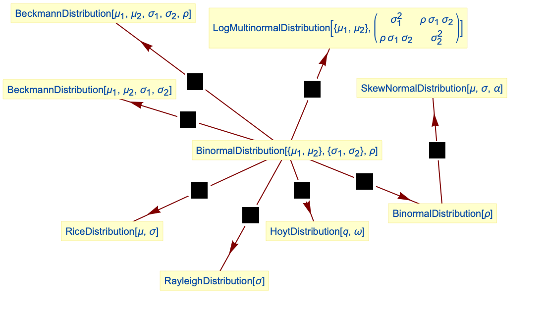
- BinormalDistributionは,数多くの他の分布と深く関係している.定義から,BinormalDistributionはNormalDistributionを2変数に拡張したものであり,したがってMultinormalDistributionの特殊ケースであると見ることができる.BinormalDistributionは,ν がInfinityに近付くに従ってMultivariateTDistribution[{{1,ρ},{ρ,1}},ν]のPDFが厳密にBinormalDistribution[{0,0},{1,1},ρ]のPDFになるという意味で,MultivariateTDistributionについての極限分布である.これに加え,BinormalDistributionを変換してSkewNormalDistributionとLogMultinormalDistributionの両方を与えることができる.二変量正規分布は,二変量正規分布に従う平均ベクトルが(0,0)で標準偏差ベクトルが

のベクトルのノルムはHoytDistribution[q,ω]に従って分布しているという意味で,HoytDistributionの構築ブロックと考えることができる.BinormalDistributionはNormalDistributionから積コピュラ分布(CopulaDistribution)を介して得ることができ,RayleighDistribution,RiceDistribution,BeckmannDistributionとも関連している.
例題
すべて開く すべて閉じる例 (4)
ParallelTable[Plot3D[PDF[BinormalDistribution[{-1, 1}, {1, 2}, ρ], {x, y}], {x, -3, 3}, {y, -6, 6}, PlotRange -> All, MeshFunctions -> {#3&}, MeshShading -> {None, Red, None, Yellow}, PlotPoints -> 25], {ρ, {-.7, -0.4, 0, 0.3, 0.5, 0.8}}]PDF[BinormalDistribution[{Subscript[μ, 1], Subscript[μ, 2]}, {Subscript[σ, 1], Subscript[σ, 2]}, ρ], {x, y}]ParallelTable[Plot3D[CDF[BinormalDistribution[{-1, 1}, {1, 2}, ρ], {x, y}], {x, -3, 3}, {y, -6, 6}, MeshFunctions -> {#3&}, MeshShading -> {None, Red, None, Yellow}, PlotPoints -> 25], {ρ, {-.7, -0.5, 0, 0.3, 0.5, 0.8}}]Mean[BinormalDistribution[{Subscript[μ, 1], Subscript[μ, 2]}, {Subscript[σ, 1], Subscript[σ, 2]}, ρ]]Variance[BinormalDistribution[{Subscript[μ, 1], Subscript[μ, 2]}, {Subscript[σ, 1], Subscript[σ, 2]}, ρ]]Covariance[BinormalDistribution[{Subscript[μ, 1], Subscript[μ, 2]}, {Subscript[σ, 1], Subscript[σ, 2]}, ρ]]スコープ (8)
sample = RandomVariate[𝒹 = BinormalDistribution[{1, 2}, {1.5, 2}, 0.6], 10 ^ 4];{Histogram3D[sample, 30, "PDF", ColorFunction -> "Rainbow", PlotRange -> {{-5, 6}, {-3, 7}, All}], Plot3D[PDF[𝒹, {x, y}], {x, -5, 6}, {y, -3, 7}, ColorFunction -> "Rainbow", PlotPoints -> 35, PlotRange -> All]}sample = RandomVariate[BinormalDistribution[{-1, 2}, {1, 2}, 0.3], 10 ^ 3];edist = EstimatedDistribution[sample, BinormalDistribution[{μ1, μ2}, {σ1, σ2}, ρ]]DistributionFitTest[sample, edist]Skewness[BinormalDistribution[{Subscript[μ, 1], Subscript[μ, 2]}, {Subscript[σ, 1], Subscript[σ, 2]}, ρ]]Kurtosis[BinormalDistribution[{Subscript[μ, 1], Subscript[μ, 2]}, {Subscript[σ, 1], Subscript[σ, 2]}, ρ]]Covariance[BinormalDistribution[ρ]]//MatrixFormCovariance[BinormalDistribution[{σ1, σ2}, ρ]]//MatrixFormCorrelation[BinormalDistribution[{σ1, σ2}, ρ]]//MatrixFormFormulaGrid[list_, type_] := Grid[...]FormulaGrid[Table[Moment[BinormalDistribution[{Subscript[μ, 1], Subscript[μ, 2]}, {Subscript[σ, 1], Subscript[σ, 2]}, ρ], {2, k}]//Simplify, {k, 0, 5}], M]FormulaGrid[Table[CentralMoment[BinormalDistribution[{Subscript[μ, 1], Subscript[μ, 2]}, {Subscript[σ, 1], Subscript[σ, 2]}, ρ], {3, k}]//Simplify, {k, 0, 5}], CM]FormulaGrid[Table[FactorialMoment[BinormalDistribution[{Subscript[μ, 1], Subscript[μ, 2]}, {Subscript[σ, 1], Subscript[σ, 2]}, ρ], {2, k}]//FullSimplify, {k, 0, 4}], FM]FormulaGrid[Table[Cumulant[BinormalDistribution[{Subscript[μ, 1], Subscript[μ, 2]}, {Subscript[σ, 1], Subscript[σ, 2]}, ρ], {2, k}], {k, 0, 5}], C]Cumulant[BinormalDistribution[{Subscript[μ, 1], Subscript[μ, 2]}, {Subscript[σ, 1], Subscript[σ, 2]}, ρ], {r, k}]ParallelTable[Plot3D[HazardFunction[BinormalDistribution[{1, 2}, {1, 2}, ρ], {x, y}], {x, -2, 7}, {y, -2, 7}, PlotRange -> All, MeshFunctions -> {#3&}, MeshShading -> {None, Red, None, Yellow}, PlotPoints -> 35, AxesLabel -> Automatic], {ρ, {-0.1, 0.3, 0.6}}]𝒟 = BinormalDistribution[{Subscript[μ, 1], Subscript[μ, 2]}, {Subscript[σ, 1], Subscript[σ, 2]}, ρ];MarginalDistribution[𝒟, 1]MarginalDistribution[𝒟, 2]母数でQuantityを一貫して使うとQuantityDistributionが与えられる:
weightHeight𝒟 = BinormalDistribution[{Quantity[85, "kg"], Quantity[182, "cm"]}, {Quantity[5, "kg"], Quantity[7, "cm"]}, 0.34]NProbability[w > ["28 kg/m^2"] h ^ 2, {w, h}weightHeight𝒟]アプリケーション (5)
CompareHistogram3D[dist_, {xmin_, xmax_, dx_}, {ymin_, ymax_, dy_}, df_ : PDF, opts___ ? OptionQ] :=
Module[{hist, dplot},
hist = Histogram3D[RandomVariate[dist, 10 ^ 4], {{xmin, xmax, dx}, {ymin, ymax, dy}}, ToString[df], PlotRange -> {{xmin, xmax}, {ymin, ymax}, All}, ChartBaseStyle -> Opacity[0.5]];
dplot = Plot3D[df[dist, {x, y}], {x, xmin, xmax}, {y, ymin, ymax}, Mesh -> {Range[xmin, xmax, dx], Range[ymin, ymax, dy]}, PlotRange -> All, MeshStyle -> Gray, PlotStyle -> Hue[.15, .7, .8]];
Show[hist, dplot]
];𝒟 = BinormalDistribution[{1, 2}, {1.5, 2}, 0.6];CompareHistogram3D[𝒟, {-5, 6, 1}, {-3, 7, 1}, PDF]CompareHistogram3D[𝒟, {-5, 6, 1}, {-3, 7, 1}, CDF]Quantity母数を使って空気の圧力と体積の両方の測定量のためのBinormalDistributionモデルを指定する:
𝒬𝒟 = BinormalDistribution[{Quantity[1.03, "Atmospheres"], Quantity[83, "Meters"^3]}, {Quantity[0.01, "Atmospheres"], Quantity[0.9, "Meters"^3]}, Quantity[13.2, "Percent"]]Subscript[𝒯, 0] = UnitConvert[Quantity[23., "Celsius"], "Kelvins"];
TransformedDistribution[(𝒫 𝒱/["ideal gas constant"]Subscript[𝒯, 0]), {𝒫, 𝒱}𝒬𝒟]{Mean[%], StandardDeviation[%]}//UnitSimplify中型車両の市街地走行時と高速道路走行時の走行可能距離は二変量正規分布に従う:
midsizeMPG2009 = QuantityArray[{{16, 22}, {18, 26}, {17, 25}, {16, 23}, {16, 23}, {14, 19}, {13, 19}, {10, 14}, {10, 17}, {18, 28}, {18, 27}, {17, 25}, {17, 25}, {17, 26}, {17, 26}, {16, 25}, {17, 25}, {15, 22}, {15, 23}, {11, 17}, {11, 17}, {17, 28}, {16, 24}, {16, 25}, {16, 25}, {17, 26}, {18, 26}, {17, 26}, {17, 25}, {17, 26}, {13, 19}, {15, 24}, {17, 26}, {15, 22}, {22, 33}, {22, 30}, {18, 29}, {17, 26}, {26, 34}, {21, 30}, {13, 20}, {19, 27}, {16, 27}, {21, 30}, {13, 20}, {19, 27}, {16, 27}, {24, 30}, {23, 27}, {23, 29}, {21, 25}, {19, 27}, {10, 15}, {9, 16}, {17, 25}, {20, 29}, {20, 28}, {18, 26}, {24, 33}, {25, 33}, {16, 25}, {15, 23}, {22, 32}, {22, 32}, {20, 28}, {23, 30}, {24, 32}, {19, 27}, {19, 26}, {18, 25}, {17, 24}, {16, 24}, {16, 23}, {16, 24}, {16, 23}, {20, 22}, {17, 25}, {20, 29}, {20, 28}, {18, 26}, {17, 24}, {18, 28}, {20, 29}, {21, 30}, {17, 25}, {18, 25}, {23, 32}, {17, 24}, {16, 22}, {15, 22}, {13, 19}, {13, 20}, {20, 27}, {16, 25}, {23, 32}, {23, 31}, {18, 27}, {19, 26}, {35, 33}, {19, 26}, {24, 30}, {21, 29}, {26, 31}, {27, 33}, {24, 32}, {11, 18}, {24, 30}, {24, 32}, {22, 33}, {17, 26}, {26, 34}, {21, 31}, {21, 31}, {19, 28}, {33, 34}, {48, 45}, {19, 29}, {15, 23}, {15, 22}, {16, 25}}, "miles per gallon"];edist = EstimatedDistribution[midsizeMPG2009, BinormalDistribution[{μ1, μ2}, {σ1, σ2}, ρ]]市街地走行時の走行可能距離が最低でも1ガロンあたり19マイル,高速道路走行時の走行可能距離が最低でも1ガロンあたり26マイルの中型車両の割合を百分率で求める:
100 SurvivalFunction[edist, {Quantity[19, "Miles"/"Gallons"], Quantity[26, "Miles"/"Gallons"]}]市街地走行時の走行可能距離が1ガロンあたり15マイル以下の車両の高速道路走行時の平均走行可能距離を求める:
NExpectation[yx ≤ Quantity[15, "Miles"/"Gallons"], {x, y}edist]市街地走行時の走行可能距離と高速道路走行時の走行可能距離の分布を示す:
Plot[Table[PDF[MarginalDistribution[edist, i], Quantity[x, "miles per gallon"]], {i, 2}]//Evaluate, {x, 10, 40}, Filling -> Axis, PlotLegends -> {"city", "highway"}, AxesLabel -> {"mpg"}]市街地走行が全体の65%を占めると仮定して走行可能距離を求める:
mixedMPG = MixtureDistribution[{.65, .35}, {MarginalDistribution[edist, 1], MarginalDistribution[edist, 2]}];Plot[PDF[mixedMPG, Quantity[x, "miles per gallon"]]//Evaluate, {x, 10, 40}, Filling -> Axis, AxesLabel -> {"mpg"}]Mean[mixedMPG]直径6cm,長さ10cmの円筒型のローラーベアリングが製造されている.品質管理は直径と長さが標準偏差が0.01cmの正規分布に従って変化することを許容する.相関係数
で長さが長くなると直径が短くなり逆もまた真であることが知られている.BinormalDistributionを使ってベアリングの体積をモデル化する:
vol = TransformedDistribution[π h (d / 2) ^ 2,
{h, d}BinormalDistribution[{Quantity[10, "Centimeters"], Quantity[6, "Centimeters"]}, {Quantity[0.01, "Centimeters"], Quantity[0.01, "Centimeters"]}, -0.3]];Mean[vol]SmoothHistogram[RandomVariate[vol, 10 ^ 5], Automatic, "PDF", AxesLabel -> Automatic, Filling -> Axis]ライオンの群れが2つ,獲物を求めて同じ地域で狩りをしている.両方の群れの週ごとの収穫は,それぞれ平均が

および
,分散が
および
のBinormalDistributionに従っている.食物を求めて競っているので,両方の群れの週ごとの収穫は,例えば

の負の相関関係にある.両方の群れが合わせて獲物を
kg得たとして,それぞれの群れの取り分を収穫サイズ
の関数として推定する:
bn = BinormalDistribution[{Subscript[μ, 1], Subscript[μ, 2]}, {Subscript[σ, 1], Subscript[σ, 2]}, ρ];
assumps = -1 < ρ < 1 && τ > 0 && Subscript[μ, 1] > Subscript[μ, 2] > 0 && Subscript[σ, 2] > Subscript[σ, 1] > 0;mean1 = Simplify[Expectation[xx + y == τ, {x, y}bn, Assumptions -> assumps]]両方の群れの獲物の合計が平均値の合計より大きい場合,最初の群れの取り分は期待値が高く分散が小さいにもかかわらず相手よりも小さい:
Refine[Reduce[(mean1/τ) < (Subscript[μ, 1]/Subscript[μ, 1] + Subscript[μ, 2]) && assumps, {τ, ρ}, Reals, Backsubstitution -> True], assumps](mean1/τ) /. {Subscript[μ, 1] -> 740, Subscript[μ, 2] -> 650, Subscript[σ, 1] -> 30, Subscript[σ, 2] -> 50, τ -> 1800} /. {{ρ -> -0.75}, {ρ -> 0.}}特性と関係 (17)
ContourPlot[PDF[BinormalDistribution[{0, 0}, {1, 2}, -0.4], {x, y}], {x, -3, 3}, {y, -4, 4}]A = (| | |
| --- | --- |
| a11 | a12 |
| a21 | a22 |);b = {b1, b2};TransformedDistribution[A.{u, v} + b, {u, v}BinormalDistribution[{μ1, μ2}, {σ1, σ2}, ρ]]//FullSimplify二変量正規分布の確率密度関数
は,偏微分方程式
を満足する:
Subscript[∂, ρ]PDF[BinormalDistribution[ρ], {x, y}] == Subscript[∂, x, y]PDF[BinormalDistribution[ρ], {x, y}]//Simplifyゆえに,累積分布関数
は
を満足し
に関して両辺を積分する:
{x, y} = {2., 1.}; {ρmin, ρmax} = {1 / 3, 2 / 3};CDF[BinormalDistribution[ρmax], {x, y}] - CDF[BinormalDistribution[ρmin], {x, y}] == NIntegrate[PDF[BinormalDistribution[ρ], {x, y}], {ρ, ρmin, ρmax}]Expectation[yx == μ + a, {x, y}BinormalDistribution[{μ, μ}, {σ, σ}, ρ]]
二変量正規分布の条件付き分布はNormalDistributionである:
mdist = MarginalDistribution[BinormalDistribution[ρ], 1]PDF[BinormalDistribution[ρ], {a, y}] / PDF[mdist, a]//FullSimplifyPDF[NormalDistribution[a ρ, Sqrt[1 - ρ^2]], y]FullSimplify[%% - %]Expectation[yx == a, {x, y}BinormalDistribution[ρ]]Expectation[y, yMarginalDistribution[BinormalDistribution[ρ], 1]]MultinormalDistributionのそれぞれの二変量周辺分布は二変量正規分布である:
Σ = (| | | |
| --------- | --------- | --------- |
| σ1^2 | ρ12 σ1 σ2 | ρ13 σ1 σ3 |
| ρ12 σ1 σ2 | σ2^2 | ρ23 σ2 σ3 |
| ρ13 σ1 σ3 | ρ23 σ2 σ3 | σ3^2 |);PDF[MarginalDistribution[MultinormalDistribution[{μ1, μ2, μ3}, Σ], {1, 2}], {x, y}]//Simplify[#, σ1 > 0 && σ2 > 0 && σ3 > 0]&PDF[BinormalDistribution[{μ1, μ2}, {σ1, σ2}, ρ12], {x, y}]% - %%//Simplify二変量正規分布はMultinormalDistributionの二次元のケースである:
PDF[BinormalDistribution[{μ1, μ2}, {σ1, σ2}, ρ], {x, y}]PDF[MultinormalDistribution[{μ1, μ2}, {{σ1 ^ 2, ρ σ1 σ2}, {ρ σ1 σ2, σ2 ^ 2}}], {x, y}]% - %%//Simplify[#, σ1 > 0 && σ2 > 0]&二変量正規分布は,
が
に近付く二次元のMultivariateTDistributionの極限である:
Limit[PDF[MultivariateTDistribution[{{1, ρ}, { ρ, 1}}, ν], {x, y}], ν -> ∞]PDF[BinormalDistribution[{0, 0}, {1, 1}, ρ], {x, y}]% - %%//SimplifyLogMultinormalDistributionはBinormalDistributionを変換したものである:
TransformedDistribution[{Exp[u], Exp[v]}, {u, v}BinormalDistribution[{Subscript[μ, 1], Subscript[μ, 2]}, {Subscript[σ, 1], Subscript[σ, 2]}, ρ]]二変量正規分布はBeckmannDistributionに関連している:
𝒟 = TransformedDistribution[Norm[{u, v}], {u, v}BinormalDistribution[{μ1, μ2}, {σ1, σ2}, ρ]];Block[{μ1 = 2, μ2 = 3, σ1 = 0.5, σ2 = 1.5, ρ = 0.7}, Show[Histogram[RandomVariate[𝒟, 10 ^ 4], 20, "PDF"], Plot[PDF[BeckmannDistribution[μ1, μ2, σ1, σ2, ρ], x], {x, 0, 10}, PlotStyle -> Thick]]]二変量正規分布はRiceDistributionに関連している:
𝒟 = TransformedDistribution[Norm[{u, v}], {u, v}BinormalDistribution[{μ / Sqrt[2], μ / Sqrt[2]}, {σ, σ}, 0]];Block[{μ = 3, σ = 2}, Show[Histogram[RandomVariate[𝒟, 10 ^ 4], 20, "PDF"], Plot[PDF[RiceDistribution[μ , σ], x], {x, 0, 12}, PlotStyle -> Thick]]]二変量正規分布はRayleighDistributionに関連している:
𝒟 = TransformedDistribution[Norm[{u, v}], {u, v}BinormalDistribution[{0, 0}, {σ, σ}, 0]];Block[{σ = 2}, Show[Histogram[RandomVariate[𝒟, 10 ^ 4], 20, "PDF"], Plot[PDF[RayleighDistribution[σ], x], {x, 0, 8}, PlotStyle -> Thick]]]HoytDistributionは二変量正規分布から得ることができる:
𝒟 = TransformedDistribution[Norm[{u, v}], {u, v}BinormalDistribution[{0, 0}, {Sqrt[ω / (1 + q ^ 2)], q Sqrt[ω / (1 + q ^ 2)]}, 0]];Block[{q = .4, ω = 2}, Show[Histogram[RandomVariate[𝒟, 10 ^ 4], 20, "ProbabilityDensity"], Plot[PDF[HoytDistribution[q, ω], x], {x, 0, 10}, PlotStyle -> Thick]]]SkewNormalDistributionはBinormalDistributionを変換したものである:
𝒟 = TransformedDistribution[u Sign[v], {u, v}BinormalDistribution[ρ]];Block[{ρ = 0.7}, Show[Histogram[RandomVariate[𝒟, 10 ^ 4], 20, "PDF"], Plot[PDF[SkewNormalDistribution[0, 1, ρ / Sqrt[1 - ρ ^ 2]], x], {x, -3, 3}, PlotStyle -> Thick]]]2つの正規分布の積コピュラ分布(CopulaDistribution)は二変量正規分布である:
𝒟 = CopulaDistribution["Product", {NormalDistribution[μ1, σ1], NormalDistribution[μ2, σ2]} ];PDF[𝒟, {x, y}]% == PDF[BinormalDistribution[{μ1, μ2}, {σ1, σ2}, 0], {x, y}]//Simplify二変量正規分布のサブカーネルと正規周辺分布を持つCopulaDistributionは二変量正規分布である:
𝒟 = CopulaDistribution[{"Binormal", ρ}, {NormalDistribution[0, σ1], NormalDistribution[0, σ2]}];PDF[𝒟, {x, y}]//FullSimplify[#, {x, y}∈Reals && σ1 > 0 && σ2 > 0 && 0 < ρ < 1]&% == PDF[BinormalDistribution[{0, 0}, {σ1, σ2}, ρ], {x, y}]//Simplify関連するガイド
テキスト
Wolfram Research (2010), BinormalDistribution, Wolfram言語関数, https://reference.wolfram.com/language/ref/BinormalDistribution.html (2016年に更新).
CMS
Wolfram Language. 2010. "BinormalDistribution." Wolfram Language & System Documentation Center. Wolfram Research. Last Modified 2016. https://reference.wolfram.com/language/ref/BinormalDistribution.html.
APA
Wolfram Language. (2010). BinormalDistribution. Wolfram Language & System Documentation Center. Retrieved from https://reference.wolfram.com/language/ref/BinormalDistribution.html
BibTeX
@misc{reference.wolfram_2026_binormaldistribution, author="Wolfram Research", title="{BinormalDistribution}", year="2016", howpublished="\url{https://reference.wolfram.com/language/ref/BinormalDistribution.html}", note=[Accessed: 09-August-2026]}
BibLaTeX
@online{reference.wolfram_2026_binormaldistribution, organization={Wolfram Research}, title={BinormalDistribution}, year={2016}, url={https://reference.wolfram.com/language/ref/BinormalDistribution.html}, note=[Accessed: 09-August-2026]}