BinormalDistribution[{μ1,μ2},{σ1,σ2},ρ]
表示均值为 {μ1,μ2}、协方差矩阵为 {{σ12,ρ σ1 σ2},{ρ σ1 σ2,σ22}} 的二元正态分布.
BinormalDistribution[{σ1,σ2},ρ]
表示均值为零的二元正态分布.
表示均值为零、协方差矩阵为 {{1,ρ },{ρ,1}} 的二元正态分布.
BinormalDistribution
BinormalDistribution[{μ1,μ2},{σ1,σ2},ρ]
表示均值为 {μ1,μ2}、协方差矩阵为 {{σ12,ρ σ1 σ2},{ρ σ1 σ2,σ22}} 的二元正态分布.
BinormalDistribution[{σ1,σ2},ρ]
表示均值为零的二元正态分布.
表示均值为零、协方差矩阵为 {{1,ρ },{ρ,1}} 的二元正态分布.
更多信息

- 在二元正态分布中,向量
的概率密度与
成正比. - BinormalDistribution 允许 μi 为任意实数,σi 为任意正实数,ρ 为 -1 到 1 之间的任意数.
- BinormalDistribution 允许 μi 和 σi 为分量方向的相同单位维度的量,ρ 为无量纲的量. »
- BinormalDistribution 可与 Mean、CDF 和 RandomVariate 等函数联合使用.
背景
- BinormalDistribution[{μ1,μ2},{σ1,σ2},ρ] 表示了一个定义在实数对上的二元(即两个变量)的统计分布,此分布的第一、第二边缘分布(MarginalDistribution)都是 NormalDistribution,即变量
和
分别满足 x1NormalDistribution[μ1,σ1] 和 x2NormalDistribution[μ2,σ2],此分布被称为二元正态分布. 因此二元正态分布有一对被称为均值向量的实数参数 (μ1,μ2),一对被称为标准差向量的正实数参数 (σ1,σ2),以及一个被称为是
和
的相关系数的实数参数
. ρ 被用于定义与该分布有关的协方差矩阵
,即一个 2×2 的矩阵,其中 
位置的元素是变量
和
之间的协方差. - 双参数形式的 BinormalDistribution[{σ1,σ2},ρ] 等价于 BinormalDistribution[{0,0},{σ1,σ2},ρ],而单参数形式的 BinormalDistribution[ρ] 等价于 BinormalDistribution[{0,0},{1,1},ρ] 且有时又被称为标准二元正态分布. 二元正态分布的随机变量有时又被称为二元正态变量. 二元正态分布有时又被称为双变量正态分布,而标准二元正态分布也被称为单位二元正态分布.
- 二元正态分布的概率密度函数(PDF)在均值

处取得绝对最大值,虽然不像单变量正态分布那样,它可能有多个“峰”. 一般而言每个相关边缘 PDF 的尾部都比较“薄”,意思是当
值较大时衰减是指数级的.(这一行为可通过研究分布的 SurvivalFunction 做精确的定量分析.) - 二元正态分布的 PDF

在满足偏微分方程
的意义下是唯一的. 与单变量正态分布的(二维意义下的)“钟形”的 PDF 不同,二元正态分布的 PDF 可能也可能不是(二维意义下的)“钟形”. 尤其,二元正态分布的 PDF 的整体形状可能会根据两个随机变量的协方差而与正态分布的 PDF 有极大的不同. 一般而言,ρ 值接近零时 PDF 看起来更“正态”(即三维意义下的钟形)而当值接近
时函数一般看起来会比较“崎岖”或“多尖”. 参数 σ1 和 σ2 决定了与之相关的一维 PDF 的尾部“厚度”,并且和 ρ 一起决定了双变量 PDF 的许多定性性质,包括其高度和“峰”的数目. - 二元正态分布在 1880 年代后期因为英国博物家弗朗西斯·高尔顿的工作而名声鹊起,他用它解释了查尔斯·达尔文著作中提到的代际变化问题. 然而此分布的种种性质早在 1808 年就已经被爱尔兰裔美国数学家 Robert Adrain 和法国数学家 Pierre-Simon Laplace 研究过了. 二元正态分布广泛存在于许多领域. 在贝叶斯分析中,均值向量和协方差矩阵的共轭先验分别是二元正态分布和逆威沙特分布. 二元正态分布可以用于检查任何一对正态分布变量之间的关系,并且由于正态分布有大量的应用,二元正态分布因此被用于模拟许多物理现象. 例如,二元正态分布有时被用于对相邻地理区域的降雨建模,以探讨其对农业的影响. 此外,一些物理属性,包括身高、体重、鞋的大小等,在人群中的分布都已知是很接近于正态分布的,由此可知,二元正态分布可以用来研究这些在同一个体上观察到的成对特性. 二元正态分布还被发现在如计算机图形学、制造和质量管理,以及气象等其它领域有应用.
- RandomVariate 可被用于给出二元正态分布的一个或多个机器精度或任意精度(后者可用 WorkingPrecision 选项指定)的伪随机变量. Distributed[{x,y},BinormalDistribution[{μ1,μ2},{σ1,σ2},ρ]],更简洁的写法是 {x,y}BinormalDistribution[{μ1,μ2},{σ1,σ2},ρ],可被用于声明随机变量对 (x,y) 是二元正态分布的. 这样一个声明之后可用在如 Probability、NProbability、Expectation 以及 NExpectation 这样的函数中.
- 概率密度函数和累积分布函数可用 PDF[BinormalDistribution[{μ1,μ2},{σ1,σ2},ρ],{x,y}] 和 CDF[BinormalDistribution[{μ1,μ2},{σ1,σ2},ρ],{x,y}] 求得. 平均数、中位数、方差、原点矩及中心矩可分别用 Mean、Median、Variance、Moment 和 CentralMoment 计算.
- DistributionFitTest 可被用于测试给定的数据集是否与二元正态分布一致,EstimatedDistribution 可被用于根据给定数据估算二元正态参数化分布,而 FindDistributionParameters 可拟合数据和二元正态分布. ProbabilityPlot 可被用于生成给定数据的 CDF 相对于符号二元正态分布的 CDF 的图线,而 QuantilePlot 可被用于生成给定数据的分位数相对于符号二元正态分布的分位数的图线.
- TransformedDistribution 可被用于表示转换的二元正态分布,CensoredDistribution 可被用于表示删截后位于上限值和下限值之间的值分布,而 TruncatedDistribution 可被用于表示截断后位于上限值和下限值之间的值分布. CopulaDistribution 可被用于建立包含了二元正态分布的高维分布,而 ProductDistribution 可被用于计算包括二元正态分布在内的,若干个独立分量分布的联合分布.
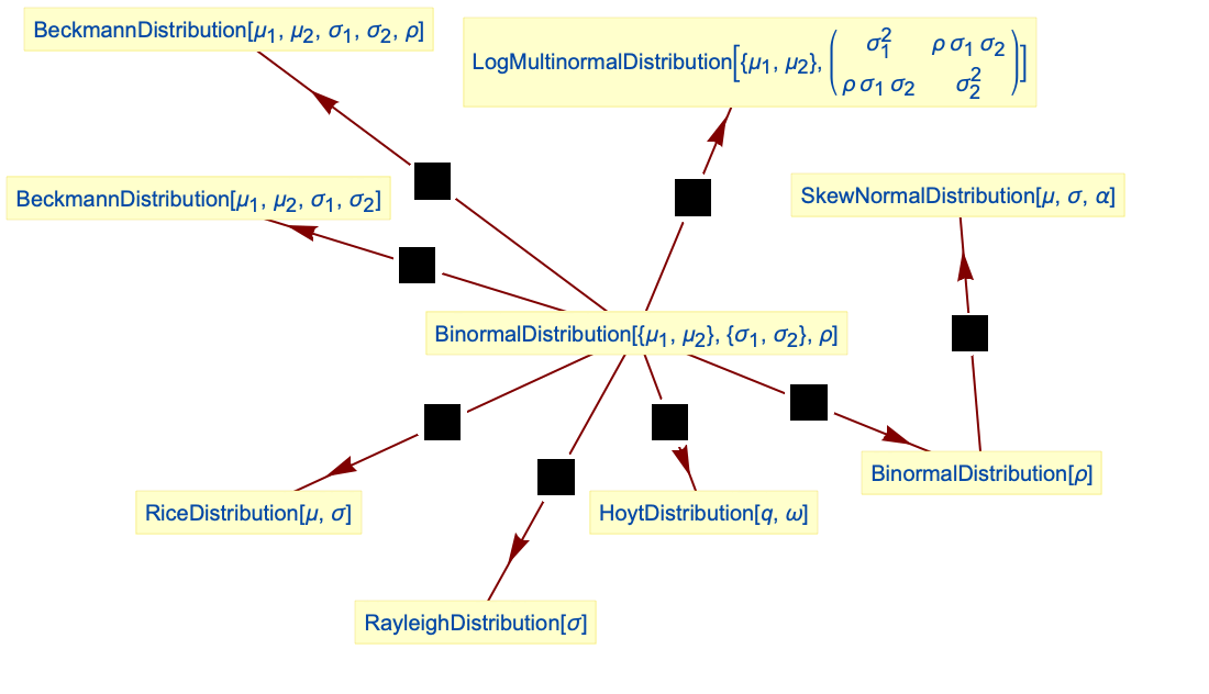
- BinormalDistribution 与许多其它分布密切相关. 由定义,BinormalDistribution 是 NormalDistribution 的双变量推广,也因此可以被看成是 MultinormalDistribution 的一个特例. BinormalDistribution 是 MultivariateTDistribution 的极限分布因为 MultivariateTDistribution[{{1,ρ},{ρ,1}},ν] 的 PDF 在 ν 趋向于 Infinity 时正是 BinormalDistribution[{0,0},{1,1},ρ] 的 PDF. 此外,BinormalDistribution 还可以被转换成 SkewNormalDistribution 和 LogMultinormalDistribution 并可以被看作是 HoytDistribution 的组成部分因为均值向量为 (0,0) 而标准差向量为

的二元正态分布向量的范数的分布为 HoytDistribution[q,ω]. BinormalDistribution 可以用 CopulaDistribution 对 NormalDistribution 做乘积得到并且还和 RayleighDistribution、RiceDistribution 以及 BeckmannDistribution 有关.
范例
打开所有单元 关闭所有单元基本范例 (4)
ParallelTable[Plot3D[PDF[BinormalDistribution[{-1, 1}, {1, 2}, ρ], {x, y}], {x, -3, 3}, {y, -6, 6}, PlotRange -> All, MeshFunctions -> {#3&}, MeshShading -> {None, Red, None, Yellow}, PlotPoints -> 25], {ρ, {-.7, -0.4, 0, 0.3, 0.5, 0.8}}]PDF[BinormalDistribution[{Subscript[μ, 1], Subscript[μ, 2]}, {Subscript[σ, 1], Subscript[σ, 2]}, ρ], {x, y}]ParallelTable[Plot3D[CDF[BinormalDistribution[{-1, 1}, {1, 2}, ρ], {x, y}], {x, -3, 3}, {y, -6, 6}, MeshFunctions -> {#3&}, MeshShading -> {None, Red, None, Yellow}, PlotPoints -> 25], {ρ, {-.7, -0.5, 0, 0.3, 0.5, 0.8}}]Mean[BinormalDistribution[{Subscript[μ, 1], Subscript[μ, 2]}, {Subscript[σ, 1], Subscript[σ, 2]}, ρ]]Variance[BinormalDistribution[{Subscript[μ, 1], Subscript[μ, 2]}, {Subscript[σ, 1], Subscript[σ, 2]}, ρ]]Covariance[BinormalDistribution[{Subscript[μ, 1], Subscript[μ, 2]}, {Subscript[σ, 1], Subscript[σ, 2]}, ρ]]范围 (8)
sample = RandomVariate[𝒹 = BinormalDistribution[{1, 2}, {1.5, 2}, 0.6], 10 ^ 4];{Histogram3D[sample, 30, "PDF", ColorFunction -> "Rainbow", PlotRange -> {{-5, 6}, {-3, 7}, All}], Plot3D[PDF[𝒹, {x, y}], {x, -5, 6}, {y, -3, 7}, ColorFunction -> "Rainbow", PlotPoints -> 35, PlotRange -> All]}sample = RandomVariate[BinormalDistribution[{-1, 2}, {1, 2}, 0.3], 10 ^ 3];edist = EstimatedDistribution[sample, BinormalDistribution[{μ1, μ2}, {σ1, σ2}, ρ]]DistributionFitTest[sample, edist]Skewness[BinormalDistribution[{Subscript[μ, 1], Subscript[μ, 2]}, {Subscript[σ, 1], Subscript[σ, 2]}, ρ]]Kurtosis[BinormalDistribution[{Subscript[μ, 1], Subscript[μ, 2]}, {Subscript[σ, 1], Subscript[σ, 2]}, ρ]]Covariance[BinormalDistribution[ρ]]//MatrixFormCovariance[BinormalDistribution[{σ1, σ2}, ρ]]//MatrixFormCorrelation[BinormalDistribution[{σ1, σ2}, ρ]]//MatrixFormFormulaGrid[list_, type_] := Grid[...]FormulaGrid[Table[Moment[BinormalDistribution[{Subscript[μ, 1], Subscript[μ, 2]}, {Subscript[σ, 1], Subscript[σ, 2]}, ρ], {2, k}]//Simplify, {k, 0, 5}], M]FormulaGrid[Table[CentralMoment[BinormalDistribution[{Subscript[μ, 1], Subscript[μ, 2]}, {Subscript[σ, 1], Subscript[σ, 2]}, ρ], {3, k}]//Simplify, {k, 0, 5}], CM]FormulaGrid[Table[FactorialMoment[BinormalDistribution[{Subscript[μ, 1], Subscript[μ, 2]}, {Subscript[σ, 1], Subscript[σ, 2]}, ρ], {2, k}]//FullSimplify, {k, 0, 4}], FM]FormulaGrid[Table[Cumulant[BinormalDistribution[{Subscript[μ, 1], Subscript[μ, 2]}, {Subscript[σ, 1], Subscript[σ, 2]}, ρ], {2, k}], {k, 0, 5}], C]Cumulant[BinormalDistribution[{Subscript[μ, 1], Subscript[μ, 2]}, {Subscript[σ, 1], Subscript[σ, 2]}, ρ], {r, k}]ParallelTable[Plot3D[HazardFunction[BinormalDistribution[{1, 2}, {1, 2}, ρ], {x, y}], {x, -2, 7}, {y, -2, 7}, PlotRange -> All, MeshFunctions -> {#3&}, MeshShading -> {None, Red, None, Yellow}, PlotPoints -> 35, AxesLabel -> Automatic], {ρ, {-0.1, 0.3, 0.6}}]𝒟 = BinormalDistribution[{Subscript[μ, 1], Subscript[μ, 2]}, {Subscript[σ, 1], Subscript[σ, 2]}, ρ];MarginalDistribution[𝒟, 1]MarginalDistribution[𝒟, 2]Quantity 在参数中的一致性使用生成 QuantityDistribution:
weightHeight𝒟 = BinormalDistribution[{Quantity[85, "kg"], Quantity[182, "cm"]}, {Quantity[5, "kg"], Quantity[7, "cm"]}, 0.34]NProbability[w > ["28 kg/m^2"] h ^ 2, {w, h}weightHeight𝒟]应用 (5)
CompareHistogram3D[dist_, {xmin_, xmax_, dx_}, {ymin_, ymax_, dy_}, df_ : PDF, opts___ ? OptionQ] :=
Module[{hist, dplot},
hist = Histogram3D[RandomVariate[dist, 10 ^ 4], {{xmin, xmax, dx}, {ymin, ymax, dy}}, ToString[df], PlotRange -> {{xmin, xmax}, {ymin, ymax}, All}, ChartBaseStyle -> Opacity[0.5]];
dplot = Plot3D[df[dist, {x, y}], {x, xmin, xmax}, {y, ymin, ymax}, Mesh -> {Range[xmin, xmax, dx], Range[ymin, ymax, dy]}, PlotRange -> All, MeshStyle -> Gray, PlotStyle -> Hue[.15, .7, .8]];
Show[hist, dplot]
];𝒟 = BinormalDistribution[{1, 2}, {1.5, 2}, 0.6];CompareHistogram3D[𝒟, {-5, 6, 1}, {-3, 7, 1}, PDF]CompareHistogram3D[𝒟, {-5, 6, 1}, {-3, 7, 1}, CDF]使用 Quantity 参数指定 BinormalDistribution 模型,用于测量气压和体积:
𝒬𝒟 = BinormalDistribution[{Quantity[1.03, "Atmospheres"], Quantity[83, "Meters"^3]}, {Quantity[0.01, "Atmospheres"], Quantity[0.9, "Meters"^3]}, Quantity[13.2, "Percent"]]Subscript[𝒯, 0] = UnitConvert[Quantity[23., "Celsius"], "Kelvins"];
TransformedDistribution[(𝒫 𝒱/["ideal gas constant"]Subscript[𝒯, 0]), {𝒫, 𝒱}𝒬𝒟]{Mean[%], StandardDeviation[%]}//UnitSimplifymidsizeMPG2009 = QuantityArray[{{16, 22}, {18, 26}, {17, 25}, {16, 23}, {16, 23}, {14, 19}, {13, 19}, {10, 14}, {10, 17}, {18, 28}, {18, 27}, {17, 25}, {17, 25}, {17, 26}, {17, 26}, {16, 25}, {17, 25}, {15, 22}, {15, 23}, {11, 17}, {11, 17}, {17, 28}, {16, 24}, {16, 25}, {16, 25}, {17, 26}, {18, 26}, {17, 26}, {17, 25}, {17, 26}, {13, 19}, {15, 24}, {17, 26}, {15, 22}, {22, 33}, {22, 30}, {18, 29}, {17, 26}, {26, 34}, {21, 30}, {13, 20}, {19, 27}, {16, 27}, {21, 30}, {13, 20}, {19, 27}, {16, 27}, {24, 30}, {23, 27}, {23, 29}, {21, 25}, {19, 27}, {10, 15}, {9, 16}, {17, 25}, {20, 29}, {20, 28}, {18, 26}, {24, 33}, {25, 33}, {16, 25}, {15, 23}, {22, 32}, {22, 32}, {20, 28}, {23, 30}, {24, 32}, {19, 27}, {19, 26}, {18, 25}, {17, 24}, {16, 24}, {16, 23}, {16, 24}, {16, 23}, {20, 22}, {17, 25}, {20, 29}, {20, 28}, {18, 26}, {17, 24}, {18, 28}, {20, 29}, {21, 30}, {17, 25}, {18, 25}, {23, 32}, {17, 24}, {16, 22}, {15, 22}, {13, 19}, {13, 20}, {20, 27}, {16, 25}, {23, 32}, {23, 31}, {18, 27}, {19, 26}, {35, 33}, {19, 26}, {24, 30}, {21, 29}, {26, 31}, {27, 33}, {24, 32}, {11, 18}, {24, 30}, {24, 32}, {22, 33}, {17, 26}, {26, 34}, {21, 31}, {21, 31}, {19, 28}, {33, 34}, {48, 45}, {19, 29}, {15, 23}, {15, 22}, {16, 25}}, "miles per gallon"];edist = EstimatedDistribution[midsizeMPG2009, BinormalDistribution[{μ1, μ2}, {σ1, σ2}, ρ]]求中型汽车市内油耗至少为19迈/加仑、高速油耗至少为26迈/加仑的比率:
100 SurvivalFunction[edist, {Quantity[19, "Miles"/"Gallons"], Quantity[26, "Miles"/"Gallons"]}]NExpectation[yx ≤ Quantity[15, "Miles"/"Gallons"], {x, y}edist]Plot[Table[PDF[MarginalDistribution[edist, i], Quantity[x, "miles per gallon"]], {i, 2}]//Evaluate, {x, 10, 40}, Filling -> Axis, PlotLegends -> {"city", "highway"}, AxesLabel -> {"mpg"}]mixedMPG = MixtureDistribution[{.65, .35}, {MarginalDistribution[edist, 1], MarginalDistribution[edist, 2]}];Plot[PDF[mixedMPG, Quantity[x, "miles per gallon"]]//Evaluate, {x, 10, 40}, Filling -> Axis, AxesLabel -> {"mpg"}]Mean[mixedMPG]制造直径为6厘米、长度为10厘米的圆柱滚子轴承. 质量控制允许直径和长度有正常的变化,标准偏差为0.01厘米. 众所周知,长度越长,对应的直径越短,反之亦然,相关系数为
. 使用 BinormalDistribution 模拟轴承的体积:
vol = TransformedDistribution[π h (d / 2) ^ 2,
{h, d}BinormalDistribution[{Quantity[10, "Centimeters"], Quantity[6, "Centimeters"]}, {Quantity[0.01, "Centimeters"], Quantity[0.01, "Centimeters"]}, -0.3]];Mean[vol]SmoothHistogram[RandomVariate[vol, 10 ^ 5], Automatic, "PDF", AxesLabel -> Automatic, Filling -> Axis]两个狮群在同一块地区捕食猎物. 它们每周捕获的猎物均服从 BinormalDistribution,其中均值为

和
,方差为
和
. 由于它们之间相互争夺猎物,每周收获是负相关的,比如为
. 假定两个狮群一共捕获的猎物重量为
,估计单个狮群的收获份额,作为猎物总重
的函数:
bn = BinormalDistribution[{Subscript[μ, 1], Subscript[μ, 2]}, {Subscript[σ, 1], Subscript[σ, 2]}, ρ];
assumps = -1 < ρ < 1 && τ > 0 && Subscript[μ, 1] > Subscript[μ, 2] > 0 && Subscript[σ, 2] > Subscript[σ, 1] > 0;mean1 = Simplify[Expectation[xx + y == τ, {x, y}bn, Assumptions -> assumps]]当两个狮群的猎物总重大于两个均值之和时,第一个狮群的收获较小,尽管其期望值较高且方差较小:
Refine[Reduce[(mean1/τ) < (Subscript[μ, 1]/Subscript[μ, 1] + Subscript[μ, 2]) && assumps, {τ, ρ}, Reals, Backsubstitution -> True], assumps](mean1/τ) /. {Subscript[μ, 1] -> 740, Subscript[μ, 2] -> 650, Subscript[σ, 1] -> 30, Subscript[σ, 2] -> 50, τ -> 1800} /. {{ρ -> -0.75}, {ρ -> 0.}}属性和关系 (17)
ContourPlot[PDF[BinormalDistribution[{0, 0}, {1, 2}, -0.4], {x, y}], {x, -3, 3}, {y, -4, 4}]A = (| | |
| --- | --- |
| a11 | a12 |
| a21 | a22 |);b = {b1, b2};TransformedDistribution[A.{u, v} + b, {u, v}BinormalDistribution[{μ1, μ2}, {σ1, σ2}, ρ]]//FullSimplifySubscript[∂, ρ]PDF[BinormalDistribution[ρ], {x, y}] == Subscript[∂, x, y]PDF[BinormalDistribution[ρ], {x, y}]//Simplify{x, y} = {2., 1.}; {ρmin, ρmax} = {1 / 3, 2 / 3};CDF[BinormalDistribution[ρmax], {x, y}] - CDF[BinormalDistribution[ρmin], {x, y}] == NIntegrate[PDF[BinormalDistribution[ρ], {x, y}], {ρ, ρmin, ρmax}]Expectation[yx == μ + a, {x, y}BinormalDistribution[{μ, μ}, {σ, σ}, ρ]]
双正态分布的条件分布是一个 NormalDistribution:
mdist = MarginalDistribution[BinormalDistribution[ρ], 1]PDF[BinormalDistribution[ρ], {a, y}] / PDF[mdist, a]//FullSimplifyPDF[NormalDistribution[a ρ, Sqrt[1 - ρ^2]], y]FullSimplify[%% - %]Expectation[yx == a, {x, y}BinormalDistribution[ρ]]Expectation[y, yMarginalDistribution[BinormalDistribution[ρ], 1]]MultinormalDistribution 的每个双正态边缘分布是双正态分布:
Σ = (| | | |
| --------- | --------- | --------- |
| σ1^2 | ρ12 σ1 σ2 | ρ13 σ1 σ3 |
| ρ12 σ1 σ2 | σ2^2 | ρ23 σ2 σ3 |
| ρ13 σ1 σ3 | ρ23 σ2 σ3 | σ3^2 |);PDF[MarginalDistribution[MultinormalDistribution[{μ1, μ2, μ3}, Σ], {1, 2}], {x, y}]//Simplify[#, σ1 > 0 && σ2 > 0 && σ3 > 0]&PDF[BinormalDistribution[{μ1, μ2}, {σ1, σ2}, ρ12], {x, y}]% - %%//Simplify双正态分布是 MultinormalDistribution 的二维情况:
PDF[BinormalDistribution[{μ1, μ2}, {σ1, σ2}, ρ], {x, y}]PDF[MultinormalDistribution[{μ1, μ2}, {{σ1 ^ 2, ρ σ1 σ2}, {ρ σ1 σ2, σ2 ^ 2}}], {x, y}]% - %%//Simplify[#, σ1 > 0 && σ2 > 0]&当
趋近于
时,双正态分布是二维 MultivariateTDistribution 的一个极限情况:
Limit[PDF[MultivariateTDistribution[{{1, ρ}, { ρ, 1}}, ν], {x, y}], ν -> ∞]PDF[BinormalDistribution[{0, 0}, {1, 1}, ρ], {x, y}]% - %%//SimplifyLogMultinormalDistribution 是 BinormalDistribution 的一个变换:
TransformedDistribution[{Exp[u], Exp[v]}, {u, v}BinormalDistribution[{Subscript[μ, 1], Subscript[μ, 2]}, {Subscript[σ, 1], Subscript[σ, 2]}, ρ]]双正态分布与 BeckmannDistribution 相关:
𝒟 = TransformedDistribution[Norm[{u, v}], {u, v}BinormalDistribution[{μ1, μ2}, {σ1, σ2}, ρ]];Block[{μ1 = 2, μ2 = 3, σ1 = 0.5, σ2 = 1.5, ρ = 0.7}, Show[Histogram[RandomVariate[𝒟, 10 ^ 4], 20, "PDF"], Plot[PDF[BeckmannDistribution[μ1, μ2, σ1, σ2, ρ], x], {x, 0, 10}, PlotStyle -> Thick]]]双正态分布与 RiceDistribution 相关:
𝒟 = TransformedDistribution[Norm[{u, v}], {u, v}BinormalDistribution[{μ / Sqrt[2], μ / Sqrt[2]}, {σ, σ}, 0]];Block[{μ = 3, σ = 2}, Show[Histogram[RandomVariate[𝒟, 10 ^ 4], 20, "PDF"], Plot[PDF[RiceDistribution[μ , σ], x], {x, 0, 12}, PlotStyle -> Thick]]]双正态分布与 RayleighDistribution 相关:
𝒟 = TransformedDistribution[Norm[{u, v}], {u, v}BinormalDistribution[{0, 0}, {σ, σ}, 0]];Block[{σ = 2}, Show[Histogram[RandomVariate[𝒟, 10 ^ 4], 20, "PDF"], Plot[PDF[RayleighDistribution[σ], x], {x, 0, 8}, PlotStyle -> Thick]]]HoytDistribution 可以从双正态分布得到:
𝒟 = TransformedDistribution[Norm[{u, v}], {u, v}BinormalDistribution[{0, 0}, {Sqrt[ω / (1 + q ^ 2)], q Sqrt[ω / (1 + q ^ 2)]}, 0]];Block[{q = .4, ω = 2}, Show[Histogram[RandomVariate[𝒟, 10 ^ 4], 20, "ProbabilityDensity"], Plot[PDF[HoytDistribution[q, ω], x], {x, 0, 10}, PlotStyle -> Thick]]]SkewNormalDistribution 是 BinormalDistribution 的一个变换:
𝒟 = TransformedDistribution[u Sign[v], {u, v}BinormalDistribution[ρ]];Block[{ρ = 0.7}, Show[Histogram[RandomVariate[𝒟, 10 ^ 4], 20, "PDF"], Plot[PDF[SkewNormalDistribution[0, 1, ρ / Sqrt[1 - ρ ^ 2]], x], {x, -3, 3}, PlotStyle -> Thick]]]两个正态分布的乘积 CopulaDistribution 是一个双正态分布:
𝒟 = CopulaDistribution["Product", {NormalDistribution[μ1, σ1], NormalDistribution[μ2, σ2]} ];PDF[𝒟, {x, y}]% == PDF[BinormalDistribution[{μ1, μ2}, {σ1, σ2}, 0], {x, y}]//Simplify含有双正态子核与正态边缘分布的 CopulaDistribution 是双正态分布:
𝒟 = CopulaDistribution[{"Binormal", ρ}, {NormalDistribution[0, σ1], NormalDistribution[0, σ2]}];PDF[𝒟, {x, y}]//FullSimplify[#, {x, y}∈Reals && σ1 > 0 && σ2 > 0 && 0 < ρ < 1]&% == PDF[BinormalDistribution[{0, 0}, {σ1, σ2}, ρ], {x, y}]//Simplify文本
Wolfram Research (2010),BinormalDistribution,Wolfram 语言函数,https://reference.wolfram.com/language/ref/BinormalDistribution.html (更新于 2016 年).
CMS
Wolfram 语言. 2010. "BinormalDistribution." Wolfram 语言与系统参考资料中心. Wolfram Research. 最新版本 2016. https://reference.wolfram.com/language/ref/BinormalDistribution.html.
APA
Wolfram 语言. (2010). BinormalDistribution. Wolfram 语言与系统参考资料中心. 追溯自 https://reference.wolfram.com/language/ref/BinormalDistribution.html 年
BibTeX
@misc{reference.wolfram_2026_binormaldistribution, author="Wolfram Research", title="{BinormalDistribution}", year="2016", howpublished="\url{https://reference.wolfram.com/language/ref/BinormalDistribution.html}", note=[Accessed: 07-August-2026]}
BibLaTeX
@online{reference.wolfram_2026_binormaldistribution, organization={Wolfram Research}, title={BinormalDistribution}, year={2016}, url={https://reference.wolfram.com/language/ref/BinormalDistribution.html}, note=[Accessed: 07-August-2026]}