


ChiDistribution
自由度 ν のカイ( )分布を表す.
詳細

- ChiDistribution[ν]は,カイ二乗 (
 )確率変数の平方根の分布を表す. »
 - ChiDistributionでは,ν は任意の正の実数でよい.
- ChiDistributionでは,ν は無次元量でよい. »
- ChiDistributionは,Mean,CDF,RandomVariate等の関数で使うことができる. »
予備知識
- ChiDistribution[ν]は,分布の自由度を表す正の値 ν でパラメータ化された統計的分布を表す.ν はカイ分布の確率密度関数(PDF)の一般的な形を決定し,PDFは ν の値によって単調減少になるか,領域の下限値に近付くにつれて特異値となり得る単一の峰(絶対最大値)を持つようになるかする.
- ChiDistributionは,カイ二乗確率変数の平方根が従う分布である.言い換えれば,
 が確率変数であり,
 (
( は「として分布」を表す)であるなら,
 である.同一正規分布に従う独立確率変数
 ,
,  , …,
, …,  の集合の総和
  もまたカイ分布に従う.カイ分布は,その統計的有意性に加え,理想気体の速度分布,さまざまな条件下での発射確度,分散液に対するレーダーの効果等,多くの科学的応用に見ることができる.
 - RandomVariateを使って,カイ分布から1つあるいは複数の機械精度あるいは任意精度の(後者はWorkingPrecisionオプションによる)擬似乱数変量を与えることができる.Distributed[x,ChiDistribution[ν]](より簡略な表記では xChiDistribution[ν])を使って,確率変数 x がカイ分布に従って分布していると宣言することができる.このような宣言は,Probability,NProbability,Expectation,NExpectation等の関数で用いることができる.
- 確率密度関数および累積分布関数は,PDF[ChiDistribution[ν],x]およびCDF[ChiDistribution[ν],x]を使って得ることができる.平均,中央値,分散,原点の周りのモーメント,中心モーメントはそれぞれ,Mean,Median,Variance,Moment,CentralMomentを使って計算することができる.
- DistributionFitTestを使って与えられたデータ集合がカイ分布と一致するかどうかを検定することが,EstimatedDistributionを使って与えられたデータからカイパラメトリック分布を推定することが,FindDistributionParametersを使ってデータをカイ分布にフィットすることが可能である.ProbabilityPlotを使って記号カイ分布のCDFに対する与えられたデータのCDFプロットを生成することができ,QuantilePlotを使って記号カイ分布の変位値に対する与えられたデータの変位値プロットを生成することができる.
- TransformedDistributionを使って変換されたカイ分布を,CensoredDistributionを使って上限値と下限値の間で打ち切られた値の分布を,TruncatedDistributionを使って上限値と下限値の間で切断された値の分布を表すことができる.CopulaDistributionを使ってカイ分布を含むより高次元の分布を構築することが,ProductDistributionを使ってカイ分布を含む独立成分分布との結合分布を計算することができる.
- ChiDistributionは多くの他の分布と密接に関係している.例えば,
 および
および  について,ChiDistribution[η]は,RayleighDistribution[η]およびMaxwellDistribution[η]とそれぞれ等しい.さらに,ChiDistributionは,XNakagamiDistribution[m,ω]が独立確率変数であれば
  である(ただしYChiDistribution[2m])という意味において,より一般的なNakagamiDistributionの特殊ケースであると見ることができる.ChiDistributionは,NoncentralChiSquareDistributionの変換として得ることができ,GammaDistribution,NormalDistribution,HalfNormalDistributionとも密接に関係している.
例題
すべて開く すべて閉じる例 (4)
スコープ (8)
サンプルの密度ヒストグラムを推定分布の確率密度関数と比較する:
極限ではカイ分布の尖度はNormalDistributionの尖度と同じになる:
無次元Quantityを使って自由度母数 ν を指定する:
特性と関係 (8)
ChiDistribution[ν]は ν->∞で正規分布に収束する:
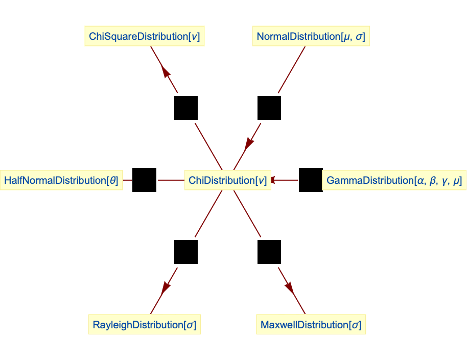
カイ変数の二乗はChiSquareDistributionに従う:
 のカイ分布は
  のHalfNormalDistributionに等しい:
 のカイ分布は
 のRayleighDistributionに等しい:
 のカイ分布は
  のMaxwellDistributionに等しい:
カイ分布はGammaDistributionの特殊ケースである:

考えられる問題 (2)

テキスト
Wolfram Research (2007), ChiDistribution, Wolfram言語関数, https://reference.wolfram.com/language/ref/ChiDistribution.html (2016年に更新).
CMS
Wolfram Language. 2007. "ChiDistribution." Wolfram Language & System Documentation Center. Wolfram Research. Last Modified 2016. https://reference.wolfram.com/language/ref/ChiDistribution.html.
APA
Wolfram Language. (2007). ChiDistribution. Wolfram Language & System Documentation Center. Retrieved from https://reference.wolfram.com/language/ref/ChiDistribution.html