ClusterClassify[data]
データを同じような要素のクラスタに分割してClassifierFunction[…]を生成する.
ClusterClassify[data,n]
n 個のクラスタでClassifierFunction[…]を生成する.
ClusterClassify
ClusterClassify[data]
データを同じような要素のクラスタに分割してClassifierFunction[…]を生成する.
ClusterClassify[data,n]
n 個のクラスタでClassifierFunction[…]を生成する.
詳細とオプション
- ClusterClassifyは,数値,テキスト,画像,日付と時点およびそれらの組合せを含むさまざまなデータタイプに使うことができる.
- クラスタの数は以下の形で指定できる.
-
Automatic クラスタ数を自動的に求める n 厳密に n 個のクラスタを求める UpTo[n] 最高で n 個のクラスタを求める - 使用可能なオプション
-
CriterionFunction Automatic メソッド選択の基準 DistanceFunction Automatic 使用する距離関数 FeatureExtractor Identity 学習するための特徴をどのように抽出するか FeatureNames Automatic 入力データに割り当てる特徴名 FeatureTypes Automatic 入力データに割り当てる特徴タイプ Method Automatic 使用するメソッド MissingValueSynthesis Automatic 欠測値の合成方法 PerformanceGoal Automatic パフォーマンスのどの面について最適化するか RandomSeeding 1234 どのような擬似乱数生成器のシードを内部的に使うべきか Weights Automatic 各例に与える重み - デフォルトで,ClusterClassifyは,DistanceFunctionが指定されていない限り自動的にデータの前処理を行う.
- DistanceFunctionの設定は,任意の距離,非類似度関数,あるいは2つの値間の距離を定義する関数 f でよい.
- PerformanceGoalの可能な設定
-
Automatic 速度,確度,メモリ間の自動トレードオフ "Memory" 分類器の必要メモリを最小にする "Quality" 分類器の確度を最大にする "Speed" 分類器の速度を最大にする "TrainingSpeed" 分類器の生成に使う時間を最小にする - Methodの可能な設定
-
Automatic メソッドを自動選択 "Agglomerate" 単一連結クラスタ化アルゴリズム "DBSCAN" 密度に基づくノイズを含むアプリケーションのクラスタ化 "GaussianMixture" ガウス混合アルゴリズムのバリエーション "JarvisPatrick" Jarvis–Patrickクラスタ化アルゴリズム "KMeans" k 平均クラスタ化アルゴリズム "KMedoids" メドイドの周りの分割 "MeanShift" 平均シフトクラスタ化アルゴリズム "NeighborhoodContraction" データ点を高密度領域にシフトさせる "SpanningTree" 最小全域木に基づいクラスタ化アルゴリズム "Spectral" スペクトルクラスタ化アルゴリズム - "KMeans"法と"KMedoids"法はクラスタ数が指定されているときにしか使用できない.
- "DBSCAN","GaussianMixture","JarvisPatrick","MeanShift","NeighborhoodContraction"の各メソッドは,クラスタ数がAutomaticのときしか使えない.
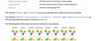
- 以下のプロットは,トイデータ集合に一般的なメソッドを適用した結果を示している.
- CriterionFunctionの可能な設定
-
"StandardDeviation" 二乗平均平方根標準偏差 "RSquared" R乗 "Dunn" Dunn指標 "CalinskiHarabasz" Calinski–Harabasz指標 "DaviesBouldin" Davies–Bouldin指標 "Silhouette" シルエットスコア Automatic 内部指標 - RandomSeedingの可能な設定
-
Automatic 関数が呼び出されるたびに自動的にシードを変える Inherited 外部シードの乱数を使う seed 明示的な整数または文字列をシードとして使う - ClusterClassify[…,FeatureExtractor"Minimal"]は,内部的な前処理はできる限り簡単にすべきであることを示している.
[image]例題
すべて開く すべて閉じる例 (3)
数値データについてClassifierFunctionを訓練する:
c = ClusterClassify[{-10, -9, -8, -7, 5, 6, 7, 8, 12}]c[0]c[0, "Probabilities"]c[{-10, 0, 30}]Plot[Values[c[x, "Probabilities"]], {x, -5, 5}]クラス数が5になるように要求し,色についてClassifierFunctionを訓練する:
SeedRandom[1234];
colors = RandomColor[70]c = ClusterClassify[colors, 5]ラベルのないデータについてClassifierFunctionを使う:
c["Red"]GatherBy[colors, c]文字列についてClassifierFunctionを訓練する:
string = {"c", "a", "bb", "dddd", "uuu7uuu", "uuuuu4u", "u5uuuuu"};c = ClusterClassify[string]components = c[string]GatherBy[string, c]スコープ (11)
data = {-10, -9, -8, -7, 5, 6, 7, 8};c = ClusterClassify[data]c[data]data = {{1.85, 1.85, 1.75, 1.6}, {0.2, 0.75, 0.1, 0.55}, {1.3, 1.9, 1.25, 1.7}, {0.25, 0.9, 0.3, 0.75}, {0.35, 0.05, 0.7, 0.35}, {0.8, 0.5, 0.7, 0.8}, {1.35, 1.45, 1.6, 1.4}, {0.75, 0.15, 0.7, 0.7}, {1.2, 1.6, 1.55, 1.5}, {1.55, 1.7, 1.95, 1.45}};c = ClusterClassify[data]c[data]SeedRandom[123];
tfdata = RandomChoice[{True, False}, {20, 3}]c = ClusterClassify[tfdata]分類器を使って新たなTrueとFalseのブールベクトルにクラスタを割り当てる:
c[{False, False, False}]分類器を使って1と0のブールベクトルにクラスタを割り当てる:
c[{0, 1, 0}]c[{{False, False, False}, {0, 1, 0}}, "Probabilities"]images = {[image], [image], [image], [image], [image], [image]};c = ClusterClassify[images, 4]Pick[images, c[images], #]& /@ Range[4]newimages = {[image], [image], [image], [image]};c[newimages]images3D = Join[Image3D /@ RandomReal[3, {3, 5, 5, 10, 2}], Image3D /@ RandomReal[1, {3, 5, 5, 3, 2}]]c = ClusterClassify[images3D]Pick[images3D, c[images3D], #]& /@ Range[2]SeedRandom[1234];
colors = RandomColor[20]c = ClusterClassify[colors, 3]c[colors]strings = DictionaryLookup["c" ~~ ___];c = ClusterClassify[strings, 10]SeedRandom[1234];
newstrings = RandomSample[DictionaryLookup["a" ~~ ___], 30];GatherBy[newstrings, c]SeedRandom[123];
data = Transpose[{RandomColor[30], RandomSample[DictionaryLookup["a" ~~ ___], 30]}]c = ClusterClassify[data, UpTo@3, Method -> "Spectral"]GatherBy[data, c]SeedRandom[1234];
data = TimeObject /@ RandomReal[AbsoluteTime[]//Round, 40]c = ClusterClassify[data, 5]Pick[data, c[data], #]& /@ Range[5]SeedRandom[1234];
data = Join[RandomReal[{-1, 1}, 20], RandomReal[{3, 4}, 20]];c = ClusterClassify[data]Information[c]Information[c, "MethodDescription"]SeedRandom[1234];
data = Join[RandomReal[{-1, 1}, {80, 2}], RandomReal[{2, 4}, {80, 2}]];
ListPlot[data]c = ClusterClassify[data]SeedRandom[1234];
datatest = RandomReal[{-1, 4}, {2000, 2}];
decision = c[datatest];ListPlot[Pick[datatest, decision, #]& /@ {1, 2}]IndeterminateThresholdを使って同じテストデータを分類する:
decision2 = c[datatest, IndeterminateThreshold -> 0.9];Indeterminateクラスタを含む結果のクラスタ化を可視化する:
ListPlot[Pick[datatest, decision2, #]& /@ {1, 2, Indeterminate}]オプション (10)
CriterionFunction (1)
circle[r_, theta_] := {r Sin[theta], r Cos[theta]};
points = RandomVariate[MixtureDistribution[{1, 1}, {UniformDistribution[{{3 / 2, 2}, {0, 2 Pi}}], UniformDistribution[{{0, 1 / 2}, {0, 2 Pi}}]}], 1000];
data = circle@@@points;
ListPlot[data, PlotRange -> All]Automatic CriterionFunctionを使って分類器関数を構築する:
c = ClusterClassify[data]Calinski–Harabasz指標をCriterionFunctionとして使って分類器関数を構築する:
d = ClusterClassify[data, CriterionFunction -> "CalinskiHarabasz"]ListPlot[GroupBy[data, ToString @* c]]ListPlot[GroupBy[data, ToString @* d]]FeatureExtractor (1)
画像のリストからClassifierFunctionを作り,新たな例を分類する:
flowers = {[image], [image], [image], [image], [image], [image], [image], [image], [image], [image], [image], [image], [image], [image], [image], [image], [image], [image], [image]};c = ClusterClassify[flowers, 3]c[{[image], [image], [image], [image]}]カスタムのFeatureExtractorを作って特徴を抽出する:
fe = FeatureExtraction[flowers, (DominantColors[#, 1]&)]d = ClusterClassify[flowers, 3, FeatureExtractor -> fe]GatherBy[flowers, d]FeatureNames (1)
c = ClusterClassify[{{2.3, "male"}, {4.8, "male"}, {9, "female"}, {5.2, "female"}, {1, "male"}, {10, "male"}, {5, "female"}}, FeatureNames -> {"age", "gender"}]c[<|"age" -> 3, "gender" -> "male"|>]c[{3, "male"}]FeatureTypes (1)
数値的な特徴タイプと名義的な特徴タイプを仮定して分類器関数を生成する:
c = ClusterClassify[{{2.3, "male"}, {4.8, "male"}, {9, "female"}, {5.2, "female"}, {1, "male"}, {10, "male"}, {5, "female"}}, FeatureTypes -> {"Numerical", "Nominal"}]d = ClusterClassify[{{2.3, "male"}, {4.8, "male"}, {9, "female"}, {5.2, "female"}, {1, "male"}, {10, "male"}, {5, "female"}}, FeatureTypes -> {"Nominal", "Nominal"}]{c[{3, " male"}], d[{3, "male"}]}Method (2)
SeedRandom[1234];
Dis = MixtureDistribution[{2, 2}, {UniformDistribution[{{-3, 3}, {-1, 0}}],
UniformDistribution[{{-3, 3}, { 2, 3}}]}];
data = RandomVariate[Dis, 1000];
ListPlot[data, PlotRange -> All]c = ClusterClassify[data]Informationを使ってメソッドの説明を得る:
Information[c, "MethodDescription"]ListPlot[Pick[data, c[data], #]& /@ {1, 2}]c = ClusterClassify[data, 2, Method -> "KMeans"]ListPlot[Pick[data, c[data], #]& /@ {1, 2}]多変量正規分布を使って大きいデータ集合を生成し,可視化する:
Dis = MixtureDistribution[{1, 1, 1, 1}, {
MultinormalDistribution[{-1, -5}, {{2, 0}, {0, 2}}],
MultinormalDistribution[{-7, 1}, {{2, 0}, {0, 2}}],
MultinormalDistribution[{2, 7}, {{1, 0}, {0, .2}}], MultinormalDistribution[{5, -20}, {{2, 0}, {0, 2}}]}];
data = RandomVariate[Dis, 70000];
ListPlot[data, PlotRange -> All]ClusterClassifyを使って使用メソッドを指定してクラスタを求め,AbsoluteTimingを見る:
{t, c} = ClusterClassify[data, 4, Method -> "KMedoids"]//AbsoluteTimingListPlot[Pick[data, c[data], #]& /@ Range[4]]ClusterClassifyを使って使用するメソッドを指定せずにクラスタを求め,AbsoluteTimingを見る:
c = ClusterClassify[data, 4]//AbsoluteTimingMissingValueSynthesis (1)
多変量正規分布を使って大きいデータ集合を生成し,可視化する:
Dis = MixtureDistribution[{1, 1, 1, 1}, {
MultinormalDistribution[{-1, -5}, {{2, 0}, {0, 2}}],
MultinormalDistribution[{-7, 1}, {{2, 0}, {0, 2}}],
MultinormalDistribution[{2, 7}, {{1, 0}, {0, .2}}], MultinormalDistribution[{5, -20}, {{2, 0}, {0, 2}}]}];
data = RandomVariate[Dis, 70000];
ListPlot[data, PlotRange -> All]ClusterClassifyを使ってクラスタを求める:
c = ClusterClassify[data, 4, Method -> "KMedoids"]c[{-3, Missing[]}, "TopProbabilities"]欠落値の合成を設定して,欠落している各変数を,既知の値が与えられた場合に推定される最も可能性の高い値に置き換える(これはデフォルトの動作である):
c[{-3, Missing[]}, "TopProbabilities", MissingValueSynthesis -> "ModeFinding"]c[{-3, Missing[]}, "TopProbabilities", MissingValueSynthesis -> "RandomSampling"]欠落している変数をランダムサンプリング戦略で繰り返し置き換えることで,点について可能性のあるクラスタの分布を取得する:
Counts[Table[c[{-3, Missing[]}, MissingValueSynthesis -> "RandomSampling"], 100]]PerformanceGoal (1)
data = Join[RandomReal[{-1 / 5, 0}, {2000, 3}], RandomReal[{0, 1 / 5}, {2000, 3}]];
ListPointPlot3D[data, PlotRange -> All]{t, d} = ClusterClassify[data, PerformanceGoal -> "TrainingSpeed"]//AbsoluteTimingクラスタをランダムに生成したデータに割り当て,AbsoluteTimingを見る:
datatest = RandomReal[{-1 / 2, 1 / 2}, {50000, 3}];d[datatest];//AbsoluteTiming{t, c} = ClusterClassify[data, PerformanceGoal -> "Speed"]//AbsoluteTimingクラスタをランダムに生成したデータに割り当て,AbsoluteTimingを上の例と比較する:
c[datatest];//AbsoluteTimingテストデータの2つのクラスタ化を可視化し,"TrainingSpeed"の設定がいかによりよい結果を与えるかを見る:
ListPointPlot3D[Pick[datatest, d[datatest], #]& /@ Range[2]]ListPointPlot3D[Pick[datatest, c[datatest], #]& /@ Range[2]]RandomSeeding (1)
colors = RandomColor[20]classifiers = Table[ClusterClassify[colors, 3], 5];新たな色について分類器を計算し,結果が常に等しいことを観察する:
#[RGBColor[0.18410183842296557, 0.8929803114282151, 0.139771903636146]]& /@ classifiersRandomSeedingオプションの値を変えて,いくつかの分類器を同じ色について訓練する:
newclassifiers = Table[ClusterClassify[colors, 3, RandomSeeding -> RandomInteger[20]], 5];分類器を
について訓練し,分類器がどのように変わるかを観察する:
#[RGBColor[0.18410183842296557, 0.8929803114282151, 0.139771903636146]]& /@ newclassifiersWeights (1)
data = Join[ Range[0, 5, 0.05], Range[25, 30, 0.05], {90}];Histogram[data]c = ClusterClassify[data]c[{20, 90}]weights = Append[ConstantArray[1, Length[data] - 1], 300];
c = ClusterClassify[data, Weights -> weights]c[{20, 90}]アプリケーション (3)
いくつかの分類器を一様分布に従う小さいデータ集合について訓練する:
SeedRandom[1234];
dataset = RandomReal[{-.5, .5}, {500, 2}];
dataset = Select[dataset, #[[1]] > #[[2]]&];classifiers = Table[ClusterClassify[dataset, n, Method -> "KMedoids"], {n, 16}];一様分布に従う多数のランダムな点についての分類器を使って三角形を分割する:
data = RandomReal[{-.5, .5}, {10 ^ 4, 2}];
data = Select[data, #[[1]] > #[[2]]&];plots = Table[ListPlot[Pick[data, (classifiers[[n]])[data], #]& /@ Range[n], AspectRatio -> 1, Frame -> True, Axes -> False, FrameTicks -> None], {n, 16}];GraphicsGrid[Partition[plots, 4], ImageSize -> Medium]SeedRandom[1234];
𝒟 = MixtureDistribution[{1, 1, 0.5}, {
MultinormalDistribution[{-1, -5}, {{2, 0}, {0, 2}}],
MultinormalDistribution[{-7, 1}, {{2, 0}, {0, 2}}],
MultinormalDistribution[{2, 7}, {{2, 0}, {0, 2}}]}];
data = RandomVariate[𝒟, 2000];
ListPlot[data, PlotRange -> All]cl = ClusterClassify[data]ListPlot[Pick[data, cl[data], #]& /@ {1, 2, 3}]c2 = ClusterClassify[data, 3]ListPlot[Pick[data, Flatten[c2[data]], #]& /@ {1, 2, 3}]image = [image];
imageData = Flatten[ImageData[ColorConvert[image, "LAB"]], 1];c = ClusterClassify[imageData, 4, Method -> "KMedoids"];decision = c[imageData];LABColor@@@(Mean /@ (Pick[imageData, decision, #]& /@ Range[4]))Image /@ ComponentMeasurements[{image, Partition[decision, 426]}, "Mask"][[All, 2]]テクニカルノート
テキスト
Wolfram Research (2016), ClusterClassify, Wolfram言語関数, https://reference.wolfram.com/language/ref/ClusterClassify.html (2020年に更新).
CMS
Wolfram Language. 2016. "ClusterClassify." Wolfram Language & System Documentation Center. Wolfram Research. Last Modified 2020. https://reference.wolfram.com/language/ref/ClusterClassify.html.
APA
Wolfram Language. (2016). ClusterClassify. Wolfram Language & System Documentation Center. Retrieved from https://reference.wolfram.com/language/ref/ClusterClassify.html
BibTeX
@misc{reference.wolfram_2026_clusterclassify, author="Wolfram Research", title="{ClusterClassify}", year="2020", howpublished="\url{https://reference.wolfram.com/language/ref/ClusterClassify.html}", note=[Accessed: 13-September-2026]}
BibLaTeX
@online{reference.wolfram_2026_clusterclassify, organization={Wolfram Research}, title={ClusterClassify}, year={2020}, url={https://reference.wolfram.com/language/ref/ClusterClassify.html}, note=[Accessed: 13-September-2026]}