DirichletCondition

DirichletCondition[beqn,pred]

方程式 beqn で表される，pred がTrueであるNDSolveおよび関連関数に渡された領域の境界の側で満足された，ディリクレ(Dirichlet)境界条件を表す．

詳細

DirichletConditionは，微分方程式とともに，DSolve，NDSolve，DEigensystem，NDEigensystem，GreenFunction等の関数における境界条件の説明に用いられる．
NDSolve[eqns,{u₁,u₂,…},{x₁,x₂,…}∈Ω]では，x_iは独立変数，u_jは従属変数，Ωは境界が∂Ωの領域である．

ディリクレ条件が指定され得る場所は青で示される．これは，領域Ωの境界 ∂Ω上（薄い青），またΩの内部境界上（濃い青）に表され得るもので，これらの点における解の値が条件 beqn を満足するように指定する．
DirichletCondition式は方程式 eqns に含まれなければならない．
独立変数 x₁, …内の方程式および不等式の任意の論理結合を pred 述部について使うことができる．
DirichletCondition[u₁r,pred]は，境界 ∂Ω上の u_iの値が r であるように指示するために使われる．一般に，境界方程式 beqn は独立変数つまり h₁ u₁+…r 内でアフィン線形でなければならない．ただし，h_iおよび r は独立変数{x₁,x₂,…}のいずれに依存してもよい．
時間依存方程式については，beqn と pred の両方が時間に依存してもよい．pred は空間的境界についてのみ考慮される．
一般に，微分方程式が一意的に可解となるためには，少なくとも1つのディリクレタイプの境界条件が指定される必要がある．ディリクレ条件は第1種境界条件とも呼ばれる．
ディリクレ条件は，pred がTrueである ∂Ωの離散化の各点で強制される．
DirichletCondition[{eqn₁,eqn₂,…},pred]は{DirichletCondition[eqn₁,pred],DirichletCondition[eqn₂,pred],…}に等しい．
DirichletCondition[eqn,{pred₁,pred₂,…}]は{DirichletCondition[eqn,pred₁],DirichletCondition[eqn,pred₂],…}に等しい．
有限要素近似の場合は，DirichletConditionは常にノードに作用し，辺や面に作用することはない．
DirichletConditionとNeumannValueは境界の同じ部分に指定されてはならない．
複数のDirichletConditionインスタンスが境界に重なってはならない．

例題

すべて開くすべて閉じる

例 (2)

単位円板上で，ディリクレ境界条件でを解く：

Wolfram Language code:

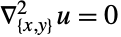
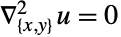
NDSolveValue[{Subsuperscript[∇, {x, y}, 2]u[x, y] == 0, DirichletCondition[u[x, y] == Sin[x y], True]}, u, {x, y}∈Disk[]]

Wolfram Language code: Plot3D[%[x, y], {x, y}∈Disk[]]

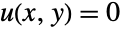
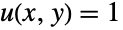
について，についてという，複数のディリクレ条件を指定する：

Wolfram Language code:

NDSolveValue[{Subsuperscript[∇, {x, y}, 2]u[x, y] == 0, DirichletCondition[u[x, y] == 0, x ≤ -0.3], DirichletCondition[u[x, y] == 1, x ≥ 0.35]}, u, {x, y}∈Disk[]]

Wolfram Language code: Plot3D[%[x, y], {x, y}∈Disk[]]

ディリクレ境界条件を使ってを単位円板上で記号的に解く：

Wolfram Language code:

DSolveValue[{Subsuperscript[∇, {x, y}, 2]u[x, y] == 0, DirichletCondition[u[x, y] == Sin[4ArcTan[x, y]], True]}, u[x, y], {x, y}∈Disk[]]

Wolfram Language code: Plot3D[%, {x, y}∈Disk[], PlotRange -> All, PlotPoints -> 101, PlotStyle -> Hue[0.55]]

スコープ (4)

穴のある領域を指定する：

Wolfram Language code:

Ω = RegionDifference[Rectangle[{-1, -1}, {1, 1}], Rectangle[{-1 / 2, -1 / 2}, {1 / 2, 1 / 2}]];
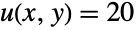
RegionPlot[Ω]

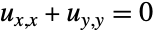
内側の境界に，外側の境界にと，複数のディリクレ条件を設定し，この領域上でラプラス(Laplace)方程式を解く：

Wolfram Language code:

NDSolveValue[{Subsuperscript[∇, {x, y}, 2]u[x, y] == 0, DirichletCondition[u[x, y] == 100., Abs[x] == 1 / 2 && -1 / 2 ≤ y ≤ 1 / 2 || -1 / 2 ≤ x ≤ 1 / 2 && Abs[y] == 1 / 2], 
	DirichletCondition[u[x, y] == 20., Abs[x] == 1 || Abs[y] == 1]}, u, {x, y}∈Ω]

Wolfram Language code: Plot3D[%[x, y], {x, y}∈Ω, Mesh -> None, PlotRange -> All]

穴がありディリクレ条件もある領域上でを解く．領域を指定する：

Wolfram Language code:

Ω = ImplicitRegion[x ^ 2 + y ^ 2 ≥ 1, {{x, -2, 2}, {y, -2, 2}}];
RegionPlot[Ω]

方程式を解く：

Wolfram Language code:

NDSolveValue[{Inactive[Div][{{2, y}, {x, 3}} . Inactive[Grad][u[x, y], {x, y}], {x, y}] == 0, DirichletCondition[u[x, y] == 0, x^2 + y^2 == 1], DirichletCondition[u[x, y] == 1, x == 2 || x == -2 || y == 2 || y == -2]}, u, {x, y}∈Ω]

解の密度をプロットする：

Wolfram Language code: DensityPlot[%[x, y], {x, y}∈Ω]

長さ d の区間の端点で0に制約された波動方程式グリーン関数を求める：

Wolfram Language code:

gf = GreenFunction[{(1/c^2)Subscript[∂, {t, 2}]u[x, t] - Subscript[∂, {x, 2}]u[x, t], DirichletCondition[u[x, t] == 0, True]}, u[x, t], {x, 0, d}, t, {y, s}]

領域内で部分的にDirichletConditionを指定する．境界メッシュを作成して可視化する：

Wolfram Language code:

Needs["NDSolve`FEM`"]
bmesh = ToBoundaryMesh["Coordinates" -> {{0, 0}, {1 / 2, 0}, {1, 0}, {1, 1}, {0, 1}, {1 / 2, 2 / 5}}, "BoundaryElements" -> {LineElement[{{1, 2}, {2, 3}, {3, 4}, {4, 5}, {5, 1}, {2, 6}}]}];
bmesh["Wireframe"]

でDirichletConditionが設定された偏微分方程式を解く：

Wolfram Language code:

mesh = ToElementMesh[bmesh];
solution = NDSolveValue[{Laplacian[u[x, y], {x, y}] == 0, u[x, 1] == 100, u[x, 0] == 0, u[1, y] == 100 y, u[0, y] == 100 y, DirichletCondition[u[x, y] == 0, x == 1 / 2 && y <= 2 / 5]}, u, {x, y}∈mesh]

解を可視化する：

Wolfram Language code: Show[ContourPlot[solution[x, y], {x, y}∈mesh, Contours -> 20], Graphics[{Green, Line[{{1 / 2, 0}, {1 / 2, 2 / 5}}]}]]

アプリケーション (11)

1D問題 (1)

からまでの領域で，およびにディリクレ条件がある微分方程式を指定する：

Wolfram Language code:

NDSolveValue[{D[-2u[x], x, x] + 3 D[u[x], x] + 10u[x] == 1, DirichletCondition[2 * u[x] == -1, x == -1], 
	DirichletCondition[3 * u[x] == 1 / 2, x == 2]}, u, {x, -1, 2}]

解をプロットする：

Wolfram Language code: Plot[%[x], {x, -1, 2}]

2D問題 (1)

境界全体におけるディリクレ境界値が0の単位円板上でポアソン(Poisson)方程式を指定する：

Wolfram Language code: NDSolveValue[{Subsuperscript[∇, {x, y}, 2]u[x, y] == 1, DirichletCondition[u[x, y] == 0, True]}, u, {x, y}∈Disk[]]

Wolfram Language code: Plot3D[%[x, y], {x, y}∈Disk[]]

3D問題 (1)

ディリクレ境界条件の単位球体上でを解く：

Wolfram Language code:

NDSolveValue[{Subsuperscript[∇, {x, y, z}, 2]u[x, y, z] == 1, DirichletCondition[u[x, y, z] == Sin[x * y * z], True]}, u[x, y, z], {x, y, z}∈Ball[]]

Wolfram Language code: SliceContourPlot3D[%, {x, y, z}∈Ball[]]

時間依存問題 (4)

初期条件と境界条件がある時間依存問題を解く：

Wolfram Language code:

pde = D[u[t, x], t, t] == D[u[t, x], x, x];
ics = {u[0, x] == Exp[-20(x) ^ 2], Derivative[1, 0][u][0, x] == 0};
bcs = {u[t, -1] == 0, u[t, 1] == 0};

Wolfram Language code: NDSolveValue[{pde, ics, bcs}, u, {t, 0, 1}, {x, -1, 1}]

Wolfram Language code: Plot3D[%[t, x], {t, 0, 1}, {x, -1, 1}, PlotRange -> All]

境界条件がディリクレ境界条件として指定された時間依存問題を解く：

Wolfram Language code: bcs = DirichletCondition[u[t, x] == 0, x == -1 || x == 1]

Wolfram Language code: NDSolveValue[{pde, ics, bcs}, u, {t, 0, 1}, {x, -1, 1}]

Wolfram Language code: Plot3D[%[t, x], {t, 0, 1}, {x, -1, 1}, PlotRange -> All]

初期条件と時間依存境界条件がある時間依存問題を解く：

Wolfram Language code:

pde = D[u[t, x], t, t] == D[u[t, x], x, x];
ics = {u[0, x] == Exp[-20(x) ^ 2], Derivative[1, 0][u][0, x] == 0};
bcs = {DirichletCondition[u[t, x] == Sin[t], x == 1], DirichletCondition[u[t, x] == 0, x == -1]}

Wolfram Language code:

NDSolveValue[{pde, ics, bcs}, u, {t, 0, π}, {x, -1, 1}, Method -> {"PDEDiscretization" -> {"MethodOfLines", {"SpatialDiscretization" -> "FiniteElement"}}}]

Wolfram Language code: Plot3D[%[t, x], {t, 0, π}, {x, -1, 1}]

初期条件と境界条件が指定された2D時間依存熱流量問題を解く：

Wolfram Language code:

ufun = NDSolveValue[{D[u[t, x, y], t] == Subsuperscript[∇, {x, y}, 2]u[t, x, y], u[0, x, y] == Sin[Pi x] Sin[Pi y], DirichletCondition[u[t, x, y] == 0, True]}, u, {t, 0, 1}, {x, 0, 1}, {y, 0, 1}, Method -> {"PDEDiscretization" -> {"MethodOfLines", {"SpatialDiscretization" -> "FiniteElement"}}}]

t==0.5における温度分布をプロットする：

Wolfram Language code: Plot3D[ufun[0.5, x, y], {x, 0, 1}, {y, 0, 1}]

急速な放散で温度分布が0に近付く様子を時間の中で見る：

Wolfram Language code: ListAnimate@Table[Plot3D[ufun[t, x, y], {x, 0, 1}, {y, 0, 1}, PlotRange -> 1], {t, 0, .25, .025}]

端がしっかりと締められた太鼓の皮の振動を見る：

Wolfram Language code:

NDSolveValue[{D[u[t, x, y], {t, 2}] == Subsuperscript[∇, {x, y}, 2]u[t, x, y], u[0, x, y] == x y Sin[Pi( x ^ 2 + y ^ 2)], Derivative[1, 0, 0][u][0, x, y] == 0, DirichletCondition[u[t, x, y] == 0, True]}, u, {t, 0, 2}, {x, y}∈Disk[]]

振動を可視化する：

Wolfram Language code: ListAnimate@Table[Plot3D[%[t, x, y], {x, y}∈Disk[], PlotRange -> 1], {t, 0, 2, .1}]

複数の境界条件 (1)

境界で領域を指定する：

Wolfram Language code:

boundaries = {-y, (1/25) - (-(3/2) + x)^2 - y^2, 1 - x^2 - y^2, x^2 + y^2 - 4, y - x * Tan[π / 8]};
Ω = ImplicitRegion[And@@(# ≤ 0& /@ boundaries), {x, y}];

領域と境界を示す：

Wolfram Language code:

Show[RegionPlot[Ω], ContourPlot[Evaluate[Thread[boundaries == 0]], {x, 0.8, 2.2}, {y, -0.2, 1.}, ContourStyle -> {Purple, Green, Red, Blue, Purple}], PlotRange -> {{0.8, 2.2}, {-0.2, 1.}}, AspectRatio -> Automatic]

気温が赤と青の境界に設定され，流束が緑の境界上に設定されたラプラス方程式を解く：

Wolfram Language code:

NDSolveValue[{-10 Subsuperscript[∇, {x, y}, 2]u[x, y] == NeumannValue[-1000., boundaries[[2]] == 0.], {DirichletCondition[u[x, y] == 200., boundaries[[3]] == 0.], 
	DirichletCondition[u[x, y] == 15., boundaries[[4]] == 0.]}}, u, {x, y}∈Ω]

Wolfram Language code:

ContourPlot[%[x, y], {x, y}∈Ω, Mesh -> None, ColorFunction -> "TemperatureMap", Contours -> 21, AspectRatio -> Automatic]

結合系の境界条件 (3)

結合微分方程式を指定する：

Wolfram Language code: pde = {D[-2 u[x], {x, 2}] + D[4 v[x], {x, 2}] + 10 v[x] == 1, D[-3 u[x], {x, 2}] + D[-1 v[x], {x, 2}] == 0};

両方の方程式にディリクレ境界条件を指定する：

Wolfram Language code:

bcs = {DirichletCondition[2 u[x] == 1, x == 0], DirichletCondition[u[x] == 0, x == 1], DirichletCondition[v[x] == 1., x == 0], DirichletCondition[v[x] == 0, x == 1]};

方程式系を解く：

Wolfram Language code: NDSolveValue[{pde, bcs}, {u[x], v[x]}, {x, 0, 1}]

解をプロットする：

Wolfram Language code: Plot[Evaluate[%], {x, 0, 1}]

結合方程式およびを指定する：

Wolfram Language code: pde = {-Subsuperscript[∇, {x, y}, 2]u[x, y] + v[x, y] == 0, -Subsuperscript[∇, {x, y}, 2]v[x, y] + u[x, y] == 0}

各従属変数に2つのディリクレ境界条件を指定する：

Wolfram Language code:

bcs = {DirichletCondition[u[x, y] == 1., x ≥ 0.9], 
	DirichletCondition[u[x, y] == 0., x ≤ -0.9], 
	DirichletCondition[v[x, y] == 2., y ≥ 0.8], 
	DirichletCondition[v[x, y] == 3., y ≤ -0.7]};

円板上で結合方程式を解く：

Wolfram Language code: NDSolveValue[{pde, bcs}, {u[x, y], v[x, y]}, {x, y}∈Disk[]]

Wolfram Language code: Plot3D[#, {x, y}∈Disk[]]& /@ %

ヤング率Yおよびポアソン比 ν で，棒の上での平面応力演算子を指定する：

Wolfram Language code:

ps = {Inactive[Div][{{0, -(Y ν/1 - ν^2)}, {-(Y (1 - ν)/2 (1 - ν^2)), 0}}.Inactive[Grad][v[x, y], {x, y}], {x, y}] + Inactive[Div][{{-(Y/1 - ν^2), 0}, {0, -(Y (1 - ν)/2 (1 - ν^2))}}.Inactive[Grad][u[x, y], {x, y}], {x, y}], Inactive[Div][{{0, -(Y (1 - ν)/2 (1 - ν^2))}, {-(Y ν/1 - ν^2), 0}}.Inactive[Grad][u[x, y], {x, y}], {x, y}] + Inactive[Div][{{-(Y (1 - ν)/2 (1 - ν^2)), 0}, {0, -(Y/1 - ν^2)}}.Inactive[Grad][v[x, y], {x, y}], {x, y}]} /. {Y -> 10 ^ 3, ν -> 33 / 100};

左端を固定され，方向を保ったまま右端を負の方向に動かされた棒の歪み（ひずみ）を計算する：

Wolfram Language code:

{uif, vif} = NDSolveValue[{ps == {0, 0}, 
	DirichletCondition[{u[x, y] == 0., v[x, y] == 0.}, x == 0], 
	DirichletCondition[v[x, y] == -0.2, x == 5], DirichletCondition[u[x, y] == 0, x == 5]
	}, {u, v}, {x, 0, 5}, {y, 0, 1}]

方向の棒の歪みの等高線プロット：

Wolfram Language code: ContourPlot[uif[x, y], {x, 0, 5}, {y, 0, 1}, ColorFunction -> "TemperatureMap", AspectRatio -> Automatic]

方向の棒の歪みの等高線プロット：

Wolfram Language code: ContourPlot[vif[x, y], {x, 0, 5}, {y, 0, 1}, ColorFunction -> "TemperatureMap", AspectRatio -> Automatic]

棒の歪みを可視化する：

Wolfram Language code:

mr = MeshRegion[uif["ElementMesh"]];
c = MeshCoordinates[mr];
Show[
	BoundaryMesh[mr], 
	HighlightMesh[MeshRegion[c + Transpose[{uif@@@c, vif@@@c}], MeshCells[mr, {2, All}]], Style[1, Red]]
	]

特性と関係 (1)

シューティング法を通して境界条件を満足する：

Wolfram Language code: NDSolveValue[{u''[x] == -x * u[x], u[0] == 0, u[4] == 1 / 2}, u[x], {x, 0, 4}, Method -> {"Shooting"}]

Wolfram Language code: Plot[%, {x, 0, 4}]

同じ方程式を有限要素法で解く：

Wolfram Language code: NDSolveValue[{u''[x] == -x * u[x], u[0] == 0, u[4] == 1 / 2}, u[x], {x, 0, 4}, Method -> {"FiniteElement"}]

Wolfram Language code: Plot[%, {x, 0, 4}]

境界条件をディリクレ条件として指定する：

Wolfram Language code:

NDSolveValue[{u''[x] == -x * u[x], DirichletCondition[u[x] == 0, x == 0], DirichletCondition[u[x] == 1 / 2, x == 4]}, u[x], {x, 0, 4}]

Wolfram Language code: Plot[%, {x, 0, 4}]

考えられる問題 (6)

少なくとも1つのディリクレ境界条件を指定することが不可欠である：

Wolfram Language code: NDSolveValue[{Subsuperscript[∇, {x, y}, 2]u[x, y] == 1}, u[x, y], {x, y}∈Disk[]]

ディリクレ条件を指定すると所望の結果が得られる：

Wolfram Language code:

NDSolveValue[{Subsuperscript[∇, {x, y}, 2]u[x, y] == 1, DirichletCondition[u[x, y] == 0, True]}, u[x, y], {x, y}∈Disk[]]

Wolfram Language code: Plot3D[%, {x, y}∈Disk[]]

Robin境界条件を不可欠の条件として指定することで十分なこともある：

Wolfram Language code:

NDSolveValue[Subsuperscript[∇, {x, y}, 2]u[x, y] == 1 + NeumannValue[3 u[x, y] + Sin[x y], True], u[x, y], {x, y}∈Disk[]]

Wolfram Language code: Plot3D[%, {x, y}∈Disk[]]

境界条件が境界との交点を持たない場合は，警告が生成され，交点を持たない境界は，可能な場合は無視される：

Wolfram Language code:

NDSolveValue[{D[-2u[x], x, x] + 3 D[u[x], x] + 10u[x] == 1, DirichletCondition[2 * u[x] == -1, x == -1], 
	DirichletCondition[3 * u[x] == 1 / 2, x == 3]}, u, {x, -1, 2}, Method -> "FiniteElement"]

境界を調整すると問題は解決する：

Wolfram Language code:

NDSolveValue[{D[-2u[x], x, x] + 3 D[u[x], x] + 10u[x] == 1, DirichletCondition[2 * u[x] == -1, x == -1], 
	DirichletCondition[3 * u[x] == 1 / 2, x == 2]}, u, {x, -1, 2}, Method -> "FiniteElement"]

Trueを述語として指定すると，内部材料境界を含むすべての境界におけるDirichletConditionの値が適用される．

内部境界を含むメッシュを生成して可視化する：

Wolfram Language code:

mesh = NDSolve`FEM`ToElementMesh[Annulus[{0, 0}, {1, 2}], "RegionHoles" -> None];
mesh["Wireframe"]

マルチマテリアル領域のための方程式を設定する：

Wolfram Language code: eqn = Inactive[Div][(If[x ^ 2 + y ^ 2 ≤ 1, -1, -5]) Inactive[Grad][u[x, y], {x, y}], {x, y}] == 1;

すべての境界における従属変数のすべての値が0に設定された方程式を解く：

Wolfram Language code: sol = NDSolveValue[{eqn, DirichletCondition[u[x, y] == 0, True]}, u, {x, y}∈mesh];

解を可視化する：

Wolfram Language code: Plot3D[sol[x, y], {x, y}∈Disk[{0, 0}, 2], PlotRange -> All]

外側境界における従属変数の値が0に設定された方程式を解く：

Wolfram Language code: sol = NDSolveValue[{eqn, DirichletCondition[u[x, y] == 0, x ^ 2 + y ^ 2 == 2 ^ 2]}, u, {x, y}∈mesh];

解を可視化する：

Wolfram Language code: Plot3D[sol[x, y], {x, y}∈Disk[{0, 0}, 2], PlotRange -> All]

Trueを述語として指定すると，空間的なすべての境界にDirichletConditionの値が適用される：

Wolfram Language code:

sol = NDSolveValue[{D[u[t, x], {t, 1}] - Laplacian[u[t, x], {x}] == 1, DirichletCondition[u[t, x] == 0, True], u[0, x] == 0}, u, {t, 0, 1}, {x, 0, 1}]

両端で境界条件が満たされていることを確認する．初期条件もまた満たされている．時間領域は空間的な境界とは見なされないので，には境界条件がない：

Wolfram Language code:

GraphicsGrid[{{Plot[sol[t, 0], {t, 0, 1}], Plot[sol[t, 1], {t, 0, 1}]}, {Plot[sol[0, x], {x, 0, 1}], Plot[sol[1, x], {x, 0, 1}]}}, ImageSize -> Medium]

NDSolveは，デフォルトで，この偏微分方程式を時間依存問題として扱う．純粋に空間的な離散化はMethod->{"PDEDiscretization"->"FiniteElement"}を使って指定できる：

Wolfram Language code:

sol = NDSolveValue[{D[u[t, x], {t, 1}] - Laplacian[u[t, x], {x}] == 1, DirichletCondition[u[t, x] == 0, True], u[0, x] == 0}, u, {t, 0, 1}, {x, 0, 1}, Method -> {"PDEDiscretization" -> "FiniteElement"}]

同じ偏微分方程式を純粋に空間的な問題として解く場合は，DirichletConditionがすべての境界に適用される：

Wolfram Language code:

GraphicsGrid[{{Plot[sol[t, 0], {t, 0, 1}], Plot[sol[t, 1], {t, 0, 1}]}, {Plot[sol[0, x], {x, 0, 1}], Plot[sol[1, x], {x, 0, 1}]}}, ImageSize -> Medium]

インポートしたメッシュあるいは生成したメッシュが数値的に不正確であることがある．例えば，目的とする領域は四角形であるのに，領域の離散化バージョンに不正確さがあって実際にはになることがある．このような場合にの形式の述語が指定されていれば，は存在しないのでエラーメッセージが生成される．次の構築された例について考える：

Wolfram Language code:

Ω = Rectangle[{10 ^ -6, 0}, {1, 1}];
NDSolveValue[{-Laplacian[u[x, y], {x, y}] == 1, DirichletCondition[u[x, y] == 0, x == 0]}, u, {x, y}∈Ω]

これに対処する方法の一つに，述語を境界としてと定式化するものがある．ここで，は境界の厚みである：

Wolfram Language code: NDSolveValue[{-Laplacian[u[x, y], {x, y}] == 1, DirichletCondition[u[x, y] == 0, x ^ 2 <= 10 ^ -6]}, u, {x, y}∈Ω]

この手法は，数値精度の問題が発生しやすい境界の円形部分のようにより複雑な述語にも使用できる．

Top

その他のラーニングリソース

テクニカルサポート

データサイエンス，金融，ビジネス

工学

科学とテクノロジー

教育のためのテクノロジー

教育イニシアチブ

使い始める

Grow Your Skills

Wolframと繋がる

大人用の教育プログラム

若者のための教育プログラム

読む

DirichletCondition

詳細

例題

例 (2)

スコープ (4)

アプリケーション (11)

1D問題 (1)

2D問題 (1)

3D問題 (1)

時間依存問題 (4)

複数の境界条件 (1)

結合系の境界条件 (3)

特性と関係 (1)

考えられる問題 (6)

テキスト

CMS

APA

BibTeX

BibLaTeX

DirichletCondition

詳細

例題

例 (2)

スコープ (4)

アプリケーション (11)

1D問題 (1)

2D問題 (1)

3D問題 (1)

時間依存問題 (4)

複数の境界条件 (1)

結合系の境界条件 (3)

特性と関係 (1)

考えられる問題 (6)

関連項目

テクニカルノート

関連するガイド

履歴

テキスト

CMS

APA

BibTeX

BibLaTeX