DirichletCondition[beqn,pred]
表示由方程 beqn 给出的狄利克雷边界条件,在给予 NDSolve 的区域上的边界部分成立,其中 pred 为 True.
DirichletCondition
DirichletCondition[beqn,pred]
表示由方程 beqn 给出的狄利克雷边界条件,在给予 NDSolve 的区域上的边界部分成立,其中 pred 为 True.
更多信息
- DirichletCondition 在诸如 DSolve、NDSolve、DEigensystem、NDEigensystem 和 GreenFunction 这样的函数中和微分方程一起使用,描述边界条件.
- 在 NDSolve[eqns,{u1,u2,…},{x1,x2,…}∈Ω] 中,xi 是自变量,uj 是因变量,而 Ω 是边界为 ∂Ω 的区域.
- 可能需要指定狄利克雷条件的位置以蓝色显示. 它们出现在区域 Ω 的边界 ∂Ω 上(以浅蓝色表示),也可能出现在 Ω 的内部边界上(以深蓝色表示),并且指定在这些点上满足条件 beqn 的解的值.
- DirichletCondition 表达式应包括在方程 eqns 中.
- 独立变量 x1、… 的等式和不等式的的任何逻辑组合都可用作谓词 pred.
- DirichletCondition[u1r,pred] 用于阐明边界 ∂Ω 上的 ui 的值应该为 r. 一般而言,边界方程 beqn 需要在因变量中呈仿射线性,即 h1 u1+…r,其中 hi 和 r 可依赖于任何独立变量 {x1,x2,…}.
- 对于含时方程,beqn 和 pred 可能依赖于时间,只在空间边界时才考虑 pred.
- 通常情况下,使微分方程具有唯一解,需要指定至少一个狄利克雷型边界条件. 狄氏条件也称为本质边界条件.
- 狄利克雷条件在 ∂Ω 离散化的每一个点上强制成立,其中 pred 为 True.
- DirichletCondition[{eqn1,eqn2,…},pred] 等价于 {DirichletCondition[eqn1,pred],DirichletCondition[eqn2,pred],…}.
- DirichletCondition[eqn,{pred1,pred2,…}] 等价于 {DirichletCondition[eqn,pred1],DirichletCondition[eqn,pred2],…}.
- 对于有限元近似法,DirichletCondition 始终在结点上进行操作,从不在边和面上进行操作.
- 不应在边界的同一部分上同时指定 DirichletCondition 和 NeumannValue .
- 多个 DirichletCondition 实例不能在边界上重叠.
范例
打开所有单元 关闭所有单元基本范例 (2)
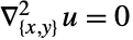
NDSolveValue[{Subsuperscript[∇, {x, y}, 2]u[x, y] == 0, DirichletCondition[u[x, y] == Sin[x y], True]}, u, {x, y}∈Disk[]]Plot3D[%[x, y], {x, y}∈Disk[]]NDSolveValue[{Subsuperscript[∇, {x, y}, 2]u[x, y] == 0, DirichletCondition[u[x, y] == 0, x ≤ -0.3], DirichletCondition[u[x, y] == 1, x ≥ 0.35]}, u, {x, y}∈Disk[]]Plot3D[%[x, y], {x, y}∈Disk[]]DSolveValue[{Subsuperscript[∇, {x, y}, 2]u[x, y] == 0, DirichletCondition[u[x, y] == Sin[4ArcTan[x, y]], True]}, u[x, y], {x, y}∈Disk[]]Plot3D[%, {x, y}∈Disk[], PlotRange -> All, PlotPoints -> 101, PlotStyle -> Hue[0.55]]范围 (4)
Ω = RegionDifference[Rectangle[{-1, -1}, {1, 1}], Rectangle[{-1 / 2, -1 / 2}, {1 / 2, 1 / 2}]];
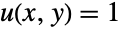
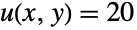
RegionPlot[Ω]设定多个狄利克雷条件,在内部边界上为
,在外部边界上为
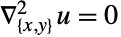
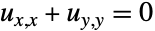
,并在该区域上求解拉普拉斯方程
:
NDSolveValue[{Subsuperscript[∇, {x, y}, 2]u[x, y] == 0, DirichletCondition[u[x, y] == 100., Abs[x] == 1 / 2 && -1 / 2 ≤ y ≤ 1 / 2 || -1 / 2 ≤ x ≤ 1 / 2 && Abs[y] == 1 / 2],
DirichletCondition[u[x, y] == 20., Abs[x] == 1 || Abs[y] == 1]}, u, {x, y}∈Ω]Plot3D[%[x, y], {x, y}∈Ω, Mesh -> None, PlotRange -> All]Ω = ImplicitRegion[x ^ 2 + y ^ 2 ≥ 1, {{x, -2, 2}, {y, -2, 2}}];
RegionPlot[Ω]NDSolveValue[{Inactive[Div][{{2, y}, {x, 3}} . Inactive[Grad][u[x, y], {x, y}], {x, y}] == 0, DirichletCondition[u[x, y] == 0, x^2 + y^2 == 1], DirichletCondition[u[x, y] == 1, x == 2 || x == -2 || y == 2 || y == -2]}, u, {x, y}∈Ω]DensityPlot[%[x, y], {x, y}∈Ω]在长度为 d 的区间上求解波动方程格林函数,在两端约束为 0:
gf = GreenFunction[{(1/c^2)Subscript[∂, {t, 2}]u[x, t] - Subscript[∂, {x, 2}]u[x, t], DirichletCondition[u[x, t] == 0, True]}, u[x, t], {x, 0, d}, t, {y, s}]在区域内部分指定一个 DirichletCondition. 创建边界网格并使之可视化:
Needs["NDSolve`FEM`"]
bmesh = ToBoundaryMesh["Coordinates" -> {{0, 0}, {1 / 2, 0}, {1, 0}, {1, 1}, {0, 1}, {1 / 2, 2 / 5}}, "BoundaryElements" -> {LineElement[{{1, 2}, {2, 3}, {3, 4}, {4, 5}, {5, 1}, {2, 6}}]}];
bmesh["Wireframe"]使用条件为
的 DirichletCondition 求解偏微分方程:
mesh = ToElementMesh[bmesh];
solution = NDSolveValue[{Laplacian[u[x, y], {x, y}] == 0, u[x, 1] == 100, u[x, 0] == 0, u[1, y] == 100 y, u[0, y] == 100 y, DirichletCondition[u[x, y] == 0, x == 1 / 2 && y <= 2 / 5]}, u, {x, y}∈mesh]Show[ContourPlot[solution[x, y], {x, y}∈mesh, Contours -> 20], Graphics[{Green, Line[{{1 / 2, 0}, {1 / 2, 2 / 5}}]}]]应用 (11)
1D 问题 (1)
2D 问题 (1)
3D 问题 (1)
时间相关问题 (4)
pde = D[u[t, x], t, t] == D[u[t, x], x, x];
ics = {u[0, x] == Exp[-20(x) ^ 2], Derivative[1, 0][u][0, x] == 0};
bcs = {u[t, -1] == 0, u[t, 1] == 0};NDSolveValue[{pde, ics, bcs}, u, {t, 0, 1}, {x, -1, 1}]Plot3D[%[t, x], {t, 0, 1}, {x, -1, 1}, PlotRange -> All]bcs = DirichletCondition[u[t, x] == 0, x == -1 || x == 1]NDSolveValue[{pde, ics, bcs}, u, {t, 0, 1}, {x, -1, 1}]Plot3D[%[t, x], {t, 0, 1}, {x, -1, 1}, PlotRange -> All]pde = D[u[t, x], t, t] == D[u[t, x], x, x];
ics = {u[0, x] == Exp[-20(x) ^ 2], Derivative[1, 0][u][0, x] == 0};
bcs = {DirichletCondition[u[t, x] == Sin[t], x == 1], DirichletCondition[u[t, x] == 0, x == -1]}NDSolveValue[{pde, ics, bcs}, u, {t, 0, π}, {x, -1, 1}, Method -> {"PDEDiscretization" -> {"MethodOfLines", {"SpatialDiscretization" -> "FiniteElement"}}}]Plot3D[%[t, x], {t, 0, π}, {x, -1, 1}]ufun = NDSolveValue[{D[u[t, x, y], t] == Subsuperscript[∇, {x, y}, 2]u[t, x, y], u[0, x, y] == Sin[Pi x] Sin[Pi y], DirichletCondition[u[t, x, y] == 0, True]}, u, {t, 0, 1}, {x, 0, 1}, {y, 0, 1}, Method -> {"PDEDiscretization" -> {"MethodOfLines", {"SpatialDiscretization" -> "FiniteElement"}}}]Plot3D[ufun[0.5, x, y], {x, 0, 1}, {y, 0, 1}]ListAnimate@Table[Plot3D[ufun[t, x, y], {x, 0, 1}, {y, 0, 1}, PlotRange -> 1], {t, 0, .25, .025}]NDSolveValue[{D[u[t, x, y], {t, 2}] == Subsuperscript[∇, {x, y}, 2]u[t, x, y], u[0, x, y] == x y Sin[Pi( x ^ 2 + y ^ 2)], Derivative[1, 0, 0][u][0, x, y] == 0, DirichletCondition[u[t, x, y] == 0, True]}, u, {t, 0, 2}, {x, y}∈Disk[]]ListAnimate@Table[Plot3D[%[t, x, y], {x, y}∈Disk[], PlotRange -> 1], {t, 0, 2, .1}]多边界条件 (1)
boundaries = {-y, (1/25) - (-(3/2) + x)^2 - y^2, 1 - x^2 - y^2, x^2 + y^2 - 4, y - x * Tan[π / 8]};
Ω = ImplicitRegion[And@@(# ≤ 0& /@ boundaries), {x, y}];Show[RegionPlot[Ω], ContourPlot[Evaluate[Thread[boundaries == 0]], {x, 0.8, 2.2}, {y, -0.2, 1.}, ContourStyle -> {Purple, Green, Red, Blue, Purple}], PlotRange -> {{0.8, 2.2}, {-0.2, 1.}}, AspectRatio -> Automatic]求解拉普拉斯方程,其中温度设在红色和蓝色边界,助熔剂在绿色边界:
NDSolveValue[{-10 Subsuperscript[∇, {x, y}, 2]u[x, y] == NeumannValue[-1000., boundaries[[2]] == 0.], {DirichletCondition[u[x, y] == 200., boundaries[[3]] == 0.],
DirichletCondition[u[x, y] == 15., boundaries[[4]] == 0.]}}, u, {x, y}∈Ω]ContourPlot[%[x, y], {x, y}∈Ω, Mesh -> None, ColorFunction -> "TemperatureMap", Contours -> 21, AspectRatio -> Automatic]耦合系统的边界条件 (3)
pde = {D[-2 u[x], {x, 2}] + D[4 v[x], {x, 2}] + 10 v[x] == 1, D[-3 u[x], {x, 2}] + D[-1 v[x], {x, 2}] == 0};bcs = {DirichletCondition[2 u[x] == 1, x == 0], DirichletCondition[u[x] == 0, x == 1], DirichletCondition[v[x] == 1., x == 0], DirichletCondition[v[x] == 0, x == 1]};NDSolveValue[{pde, bcs}, {u[x], v[x]}, {x, 0, 1}]Plot[Evaluate[%], {x, 0, 1}]pde = {-Subsuperscript[∇, {x, y}, 2]u[x, y] + v[x, y] == 0, -Subsuperscript[∇, {x, y}, 2]v[x, y] + u[x, y] == 0}bcs = {DirichletCondition[u[x, y] == 1., x ≥ 0.9],
DirichletCondition[u[x, y] == 0., x ≤ -0.9],
DirichletCondition[v[x, y] == 2., y ≥ 0.8],
DirichletCondition[v[x, y] == 3., y ≤ -0.7]};NDSolveValue[{pde, bcs}, {u[x, y], v[x, y]}, {x, y}∈Disk[]]Plot3D[#, {x, y}∈Disk[]]& /@ %指定一个平面应力运算符,其中杨氏模量 Y 和泊松比 ν 在一个条上:
ps = {Inactive[Div][{{0, -(Y ν/1 - ν^2)}, {-(Y (1 - ν)/2 (1 - ν^2)), 0}}.Inactive[Grad][v[x, y], {x, y}], {x, y}] + Inactive[Div][{{-(Y/1 - ν^2), 0}, {0, -(Y (1 - ν)/2 (1 - ν^2))}}.Inactive[Grad][u[x, y], {x, y}], {x, y}], Inactive[Div][{{0, -(Y (1 - ν)/2 (1 - ν^2))}, {-(Y ν/1 - ν^2), 0}}.Inactive[Grad][u[x, y], {x, y}], {x, y}] + Inactive[Div][{{-(Y (1 - ν)/2 (1 - ν^2)), 0}, {0, -(Y/1 - ν^2)}}.Inactive[Grad][v[x, y], {x, y}], {x, y}]} /. {Y -> 10 ^ 3, ν -> 33 / 100};计算一个杆的形变,其中左侧边缘固定,从右侧边缘移动到
方向的相反位置上,但保持其
方向:
{uif, vif} = NDSolveValue[{ps == {0, 0},
DirichletCondition[{u[x, y] == 0., v[x, y] == 0.}, x == 0],
DirichletCondition[v[x, y] == -0.2, x == 5], DirichletCondition[u[x, y] == 0, x == 5]
}, {u, v}, {x, 0, 5}, {y, 0, 1}]ContourPlot[uif[x, y], {x, 0, 5}, {y, 0, 1}, ColorFunction -> "TemperatureMap", AspectRatio -> Automatic]ContourPlot[vif[x, y], {x, 0, 5}, {y, 0, 1}, ColorFunction -> "TemperatureMap", AspectRatio -> Automatic]mr = MeshRegion[uif["ElementMesh"]];
c = MeshCoordinates[mr];
Show[
BoundaryMesh[mr],
HighlightMesh[MeshRegion[c + Transpose[{uif@@@c, vif@@@c}], MeshCells[mr, {2, All}]], Style[1, Red]]
]属性和关系 (1)
NDSolveValue[{u''[x] == -x * u[x], u[0] == 0, u[4] == 1 / 2}, u[x], {x, 0, 4}, Method -> {"Shooting"}]Plot[%, {x, 0, 4}]NDSolveValue[{u''[x] == -x * u[x], u[0] == 0, u[4] == 1 / 2}, u[x], {x, 0, 4}, Method -> {"FiniteElement"}]Plot[%, {x, 0, 4}]NDSolveValue[{u''[x] == -x * u[x], DirichletCondition[u[x] == 0, x == 0], DirichletCondition[u[x] == 1 / 2, x == 4]}, u[x], {x, 0, 4}]Plot[%, {x, 0, 4}]可能存在的问题 (6)
NDSolveValue[{Subsuperscript[∇, {x, y}, 2]u[x, y] == 1}, u[x, y], {x, y}∈Disk[]]NDSolveValue[{Subsuperscript[∇, {x, y}, 2]u[x, y] == 1, DirichletCondition[u[x, y] == 0, True]}, u[x, y], {x, y}∈Disk[]]Plot3D[%, {x, y}∈Disk[]]NDSolveValue[Subsuperscript[∇, {x, y}, 2]u[x, y] == 1 + NeumannValue[3 u[x, y] + Sin[x y], True], u[x, y], {x, y}∈Disk[]]Plot3D[%, {x, y}∈Disk[]]当边界条件与边界不相交时,将会产生一个警告,并在可能时忽略非相交边界:
NDSolveValue[{D[-2u[x], x, x] + 3 D[u[x], x] + 10u[x] == 1, DirichletCondition[2 * u[x] == -1, x == -1],
DirichletCondition[3 * u[x] == 1 / 2, x == 3]}, u, {x, -1, 2}, Method -> "FiniteElement"]NDSolveValue[{D[-2u[x], x, x] + 3 D[u[x], x] + 10u[x] == 1, DirichletCondition[2 * u[x] == -1, x == -1],
DirichletCondition[3 * u[x] == 1 / 2, x == 2]}, u, {x, -1, 2}, Method -> "FiniteElement"]如果指定 True 作为谓词,将会把 DirichletCondition 的值应用于所有边界,包括内部材料的边界.
mesh = NDSolve`FEM`ToElementMesh[Annulus[{0, 0}, {1, 2}], "RegionHoles" -> None];
mesh["Wireframe"]eqn = Inactive[Div][(If[x ^ 2 + y ^ 2 ≤ 1, -1, -5]) Inactive[Grad][u[x, y], {x, y}], {x, y}] == 1;sol = NDSolveValue[{eqn, DirichletCondition[u[x, y] == 0, True]}, u, {x, y}∈mesh];Plot3D[sol[x, y], {x, y}∈Disk[{0, 0}, 2], PlotRange -> All]sol = NDSolveValue[{eqn, DirichletCondition[u[x, y] == 0, x ^ 2 + y ^ 2 == 2 ^ 2]}, u, {x, y}∈mesh];Plot3D[sol[x, y], {x, y}∈Disk[{0, 0}, 2], PlotRange -> All]如果指定 True 作为谓词,将在所有空间边界上应用 DirichletCondition 的值:
sol = NDSolveValue[{D[u[t, x], {t, 1}] - Laplacian[u[t, x], {x}] == 1, DirichletCondition[u[t, x] == 0, True], u[0, x] == 0}, u, {t, 0, 1}, {x, 0, 1}]两端满足边界条件,初始条件也得到满足. 在
时没有边界条件,因为时域不被视为空间边界:
GraphicsGrid[{{Plot[sol[t, 0], {t, 0, 1}], Plot[sol[t, 1], {t, 0, 1}]}, {Plot[sol[0, x], {x, 0, 1}], Plot[sol[1, x], {x, 0, 1}]}}, ImageSize -> Medium]默认情况下,NDSolve 将 PDE 视为含时问题. 可用 Method->{"PDEDiscretization"->"FiniteElement"} 指定纯空间离散化:

sol = NDSolveValue[{D[u[t, x], {t, 1}] - Laplacian[u[t, x], {x}] == 1, DirichletCondition[u[t, x] == 0, True], u[0, x] == 0}, u, {t, 0, 1}, {x, 0, 1}, Method -> {"PDEDiscretization" -> "FiniteElement"}]如果将同一个 PDE 作为纯空间问题求解,则已在所有边界处应用了 DirichletCondition:
GraphicsGrid[{{Plot[sol[t, 0], {t, 0, 1}], Plot[sol[t, 1], {t, 0, 1}]}, {Plot[sol[0, x], {x, 0, 1}], Plot[sol[1, x], {x, 0, 1}]}}, ImageSize -> Medium]有时,导入的网格或甚至生成的网格都可能存在数值上的不精确. 例如,目标区域是一个矩形
,但该区域的离散化版本存在不精确性,实际上是
. 在这种情况下,如果指定了
形式的谓词,就会产生一条错误信息,因为
并不存在. 请看这个构造的例子:
Ω = Rectangle[{10 ^ -6, 0}, {1, 1}];
NDSolveValue[{-Laplacian[u[x, y], {x, y}] == 1, DirichletCondition[u[x, y] == 0, x == 0]}, u, {x, y}∈Ω]处理这种情况的一种方法是将谓词表述为一个界限:
,其中
是界限的粗细:
NDSolveValue[{-Laplacian[u[x, y], {x, y}] == 1, DirichletCondition[u[x, y] == 0, x ^ 2 <= 10 ^ -6]}, u, {x, y}∈Ω]技术笔记
-
▪
- PDE 模型概览
相关指南
-
▪
- 偏微分方程 ▪
- 微分方程 ▪
- 区域上的求解器 ▪
- 流体动力学 PDE 以及边界条件 ▪
- 偏微分方程术语 ▪
- 质量传输 PDE 和边界条件 ▪
- 固体力学 PDE 和边界条件 ▪
- 热传递 PDE 和边界条件 ▪
- 声学 PDE 和边界条件 ▪
- 电磁偏微分方程以及边界条件
文本
Wolfram Research (2014),DirichletCondition,Wolfram 语言函数,https://reference.wolfram.com/language/ref/DirichletCondition.html (更新于 2022 年).
CMS
Wolfram 语言. 2014. "DirichletCondition." Wolfram 语言与系统参考资料中心. Wolfram Research. 最新版本 2022. https://reference.wolfram.com/language/ref/DirichletCondition.html.
APA
Wolfram 语言. (2014). DirichletCondition. Wolfram 语言与系统参考资料中心. 追溯自 https://reference.wolfram.com/language/ref/DirichletCondition.html 年
BibTeX
@misc{reference.wolfram_2026_dirichletcondition, author="Wolfram Research", title="{DirichletCondition}", year="2022", howpublished="\url{https://reference.wolfram.com/language/ref/DirichletCondition.html}", note=[Accessed: 10-September-2026]}
BibLaTeX
@online{reference.wolfram_2026_dirichletcondition, organization={Wolfram Research}, title={DirichletCondition}, year={2022}, url={https://reference.wolfram.com/language/ref/DirichletCondition.html}, note=[Accessed: 10-September-2026]}