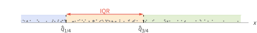
InterquartileRange[data]
data の要素における上位四分位点と下位四分位点の差 ![]() を与える.
を与える.
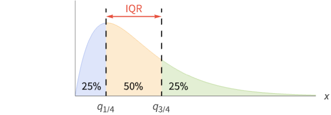
InterquartileRange[dist]
分布 dist について上位四分位点と下位四分位点の差 ![]() を与える.
を与える.


InterquartileRange
InterquartileRange[data]
data の要素における上位四分位点と下位四分位点の差 ![]() を与える.
を与える.
InterquartileRange[data,{{a,b},{c,d}}]
パラメータ a, b, c, d によって指定された四分位定義を使う.
InterquartileRange[dist]
分布 dist について上位四分位点と下位四分位点の差 ![]() を与える.
を与える.
詳細
- InterquartileRangeはIQRとしても知られている.
- InterquartileRangeは分散についての強力な測度である.これは,外れ値にはあまり敏感ではないことを意味する.
- InterquartileRange[data]は
 によって与えられる.ただし,
 はQuartiles[data]で与えられる. »
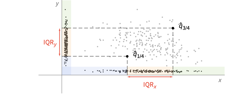
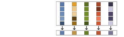
 - MatrixQ data については,四分位範囲は各列ベクトルについて計算される.InterquartileRange[{{x1,y1,…},{x2,y2,…},…}]は{InterquartileRange[{x1,x2,…}],InterquartileRange[{y1,y2,…}]}に等しい. »
- ArrayQ data については,四分位範囲はArrayReduce[InterquartileRange,data,1]に等しい. »
- InterquartileRange[data,{{a,b},{c,d}}]は,母数 a, b, c, d によって定義されるQuartilesを使う.
- 一般的に選ばれる母数{{a,b},{c,d}}には以下がある.
-
{{0, 0}, {1, 0}} 経験的な累積分布関数の逆関数(デフォルト) {{0, 0}, {0, 1}} 線形補間(カリフォルニア法) {{1/2, 0}, {0, 0}} p n に最も近い番号が付いた要素 {{1/2, 0}, {0, 1}} 線形補間(水文学者法,デフォルト) {{0, 1}, {0, 1}} 平均ベースの推定(ワイブル法) {{1, -1}, {0, 1}} 最頻値ベースの推定 {{1/3, 1/3}, {0, 1}} 中央値ベースの推定 {{3/8, 1/4}, {0, 1}} 正規分布の推定 - 母数のデフォルトによる選択値は{{1/2,0},{0,1}}である. »
- data は次の追加的な形式と解釈を持つことがある.
-
Association 値(キーは無視される) » SparseArray 配列として,Normal[data]に等しい » QuantityArray 配列としての数量 » WeightedData もとになっているEmpiricalDistributionに基づく » EventData もとになっているSurvivalDistributionに基づく » TimeSeries, TemporalData, … ベクトルまたは値の配列(タイムスタンプは無視される) » Image,Image3D RGBチャンネル値またはグレースケールの強度値 » Audio 全チャンネルの振幅値 » DateObject, TimeObject 日付のリストまたは時間のリスト » - InterquartileRange[dist]は
 によって与えられる.ただし,
 はQuartiles[dist]によって与えられる. »
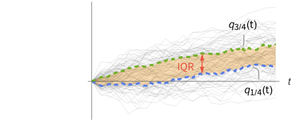
 - ランダム過程 proc については,四分位範囲関数は時点 t におけるスライス分布SliceDistribution[proc,t]についてInterquartileRange[SliceDistribution[proc,t]]として計算できる. »
例題
すべて開く すべて閉じる例 (3)
スコープ (22)
基本的な用法 (8)
InterquartileRange[{1, 2, 3, 4}]InterquartileRange[{π, E, 2}]//TogetherInterquartileRange[{1., 2., 3., 4.}]InterquartileRange[N[{1, 2, 3, 4}, 30]]InterquartileRange[{-1, 5, 10, 4, 25, 2, 1}]InterquartileRange[{-1, 5, 10, 4, 25, 2, 1}, {{0, 0}, {1, 0}}]WeightedDataの四分位範囲を求める:
InterquartileRange[WeightedData[{1, 2, 3}, {3, 7, 4}]]data = {8, 3, 5, 4, 9, 0, 4, 2, 2, 3};
weights = {0.15, 0.09, 0.12, 0.10, 0.16, 0., 0.11, 0.08, 0.08, 0.09};InterquartileRange[WeightedData[data, weights]]EventDataの四分位範囲を求める:
e = {1.0, 2.1, 3.2, 4.5, 5.7};
ci = {0, 0, 0, 1, 0};InterquartileRange[EventData[e, ci]]TemporalDataの四分位範囲を求める:
s1 = {2, 1, 6, 5, 7, 4};
s2 = {4, 7, 5, 6, 1, 2};
t = {1, 2, 5, 10, 12, 15};td = TemporalData[{s1, s2}, {t}];InterquartileRange[td[10]]TimeSeriesの四分位範囲を求める:
InterquartileRange[TemporalData[TimeSeries, {{{2.3, 1.2, 6.7, 5.8, 7.1, 4.6}}, {{0, 5, 1}}, 1, {"Discrete", 1},
{"Discrete", 1}, 1, {}}, False, 10.]]InterquartileRange[TemporalData[TimeSeries, {{{2.3, 1.2, 6.7, 5.8, 7.1, 4.6}}, {{0, 5, 1}}, 1, {"Discrete", 1},
{"Discrete", 1}, 1, {}}, False, 10.]["Values"]]data = Quantity[RandomReal[1, 6], "Meters"]InterquartileRange[data]配列データ (5)
行列のInterquartileRangeは列ごとの範囲を与える:
InterquartileRange[{{3, 5}, {1, 8}, {5, 6}, {7, 8}, {2, 4}}]InterquartileRange[RandomReal[1, {10, 2, 3}]]InterquartileRange[RandomReal[1, 10 ^ 7]]InterquartileRange[RandomReal[1, {10 ^ 6, 5}]]InterquartileRangeは,入力がAssociationのときはその値に作用する:
mat = RandomReal[1, {3, 2}];
assoc = AssociationThread[Range[3], mat]InterquartileRange[assoc]SparseArrayデータは密な配列と同じように使うことができる:
sp = SparseArray[{{i_, i_} :> i, {i_, j_} /; j < i :> (i + j) ^ 2}, {100, 10}]InterquartileRange[sp]QuantityArrayの四分位範囲を求める:
data = QuantityArray[RandomReal[1, 6], "Pounds"]InterquartileRange[data]画像データと音声データ (2)
日付と時間 (4)
dates = WolframLanguageData[All, "DateIntroduced"];DateHistogram[dates]InterquartileRange[dates]UnitConvert[%, "Years"]dates = RandomDate[4]weights = {1, 1, 1, 3};InterquartileRange[WeightedData[dates, weights]]InterquartileRange[dates]UnitConvert[%, "Days"]dates = {DateObject[{2024, 2, 29}, CalendarType -> "Julian"], DateObject[{1524, 1, 1}, CalendarType -> "Islamic"], DateObject[{6024, 1, 15}, CalendarType -> "Jewish"]}InterquartileRange[dates]UnitConvert[%, "Years"]RandomTime[3]InterquartileRange[%]{TimeObject[{12}, TimeZone -> 0], TimeObject[{12}, TimeZone -> 2], TimeObject[{12}, TimeZone -> "Asia/Tokyo"]}InterquartileRange[%]分布と過程 (3)
InterquartileRange[NormalDistribution[μ, σ]]InterquartileRange[TransformedDistribution[x^2, xNormalDistribution[]]]data = RandomVariate[NormalDistribution[], 10 ^ 3];InterquartileRange[HistogramDistribution[data]]InterquartileRange[PoissonProcess[3][6]]アプリケーション (6)
InterquartileRangeは値の広がりを示す:
dists = {NormalDistribution[0, 1], NormalDistribution[0, 2], NormalDistribution[0, 4]};Table[Plot[PDF[𝒟, x], {x, -10, 10}, Filling -> Axis, Ticks -> {Automatic, None}, PlotRange -> {Automatic, {0, 0.4}}, PlotLabel -> N@InterquartileRange[𝒟]], {𝒟, dists}]InterquartileRangeを使ってデータと分布の一致をチェックすることができる:
𝒟 = KumaraswamyDistribution[2, 3];data = RandomVariate[𝒟, 10 ^ 3];InterquartileRange[data]InterquartileRange[𝒟]N[%]年間移動四分位範囲を使って,株式データでボラティリティが高かった期間を特定する:
data = TemporalData[«4»];smooth = MovingMap[InterquartileRange, data, {Quantity[365, "Day"]}];DateListPlot[smooth]切り倒された31本のアメリカ桜について,材木の胴回り,高さ,体積の四分位間の範囲を求める:
data = ExampleData[{"Statistics", "BlackCherryTrees"}];Length[data]ListLinePlot[Transpose[data], PlotLegends -> {"Girth", "Height", "Volume"}]TableForm[{InterquartileRange[data]}, TableHeadings -> {{"Interquartile Range"}, {"Girth", "Height", "Volume"}}]ランダム過程の経路集合のスライスについて,InterquartileRangeを計算する:
data = RandomFunction[WienerProcess[], {0, 1, .01}, 10 ^ 3];times = Range[0, 1, .1];range = Map[{#, InterquartileRange[data[#]]}&, times];ListPlot[range]heights = Quantity[{134, 143, 131, 140, 145, 136, 131, 136, 143, 136, 133, 145, 147,
150, 150, 146, 137, 143, 132, 142, 145, 136, 144, 135, 141}, "Centimeters"];ListPlot[heights, Filling -> Axis, AxesLabel -> Automatic](ir = InterquartileRange[heights])//Nm = Median[heights];
n = Length[heights];
ListPlot[{heights, {{0, m}, {n, m}}, {{0, m - ir}, {n, m - ir}}, {{0, m + ir}, {n, m + ir}}}, Filling -> {1 -> 0, 3 -> {4}}, Joined -> {False, True, True, True}, PlotStyle -> {Automatic, Automatic, Gray, Gray}, PlotLegends -> {"身長", "中央値", "四分位範囲"}, AxesLabel -> Automatic]特性と関係 (4)
InterquartileRangeは,線形に補間されたQuantileの値の差分である:
data = RandomReal[10, 20];Apply[Subtract, Quantile[data, {3 / 4, 1 / 4}, {{1 / 2, 0}, {0, 1}}]]InterquartileRange[data]InterquartileRangeは,第1四分位数と第3四分位数の差である:
data = RandomReal[10, 20];qrs = Quartiles[data];
qrs[[3]] - qrs[[1]]InterquartileRange[data]QuartileDeviationは四分位範囲の半分である:
data = RandomReal[10, 20];2QuartileDeviation[data]InterquartileRange[data]BoxWhiskerChartは,データの四分位範囲を示す:
BoxWhiskerChart[RandomVariate[NormalDistribution[0, 1], 100]]考えられる問題 (1)
InterquartileRangeは数値 data を必要とする:
InterquartileRange[{a, b, c}]InterquartileRange[NormalDistribution[μ, σ]]おもしろい例題 (1)
20個,100個,300個のサンプルについてのInterquartileRange推定値の分布:
InterquartileRange[ExponentialDistribution[0.9]]SmoothHistogram[Table[InterquartileRange[RandomVariate[ExponentialDistribution[0.9], {s, 1000}]], {s, {20, 100, 300}}], Filling -> Axis, PlotLegends -> {20, 100, 300}, PlotRange -> {{0, 3}, Automatic}]テキスト
Wolfram Research (2007), InterquartileRange, Wolfram言語関数, https://reference.wolfram.com/language/ref/InterquartileRange.html (2024年に更新).
CMS
Wolfram Language. 2007. "InterquartileRange." Wolfram Language & System Documentation Center. Wolfram Research. Last Modified 2024. https://reference.wolfram.com/language/ref/InterquartileRange.html.
APA
Wolfram Language. (2007). InterquartileRange. Wolfram Language & System Documentation Center. Retrieved from https://reference.wolfram.com/language/ref/InterquartileRange.html