



NArgMin
詳細とオプション
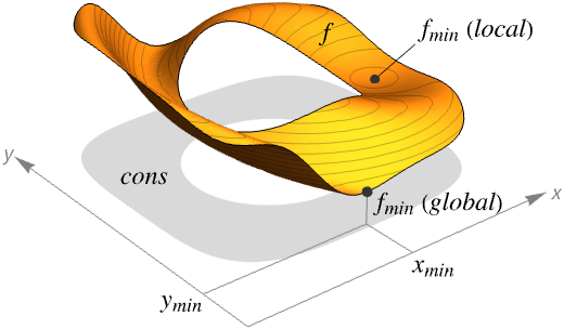
- NArgMinは大域的最適化(GO)としても知られている.
- NArgMinは,与えられた制約条件に従って常に f の最小値を求めようとする.
- NArgMinは,通常,制約が与えられた場合に可能な最小値を求めるために使われる.分野によっては,最適な戦略,最良適合,最適な構成等と呼ばれることがある.
- NArgMinは{xmin,ymin,…}の形のリストを返す.
- NArgMin[…,{x,y,…}]は事実上{x,y,…}/.Last[NMinimize[…,{x,y,…},…]]に等しい.
- f と cons が線形または凸のとき,NArgMinが与える結果は実数および整数値の両方の上で最小値になる.それ以外の場合の結果は単に極小値であるかもしれない.
- NArgMinが制約条件を満足できないと判断した場合は{Indeterminate,…}が返される.
- NArgMinは,目的関数 f と制約条件 cons がスカラー変数またはベクトル変数に依存する式で与えられるモデリング言語をサポートする.f と cons は,一般に,非常に効率的な形に解析されるが,f と cons の項が変数の数値に対して数値を与える限りNArgMinはしばしば解を求めることができる.
- 制約条件 cons は以下の論理結合でよい.
-
lhs==rhs 等式 lhs>rhs, lhs≥rhs, lhs<rhs, lhs≤rhs 不等式 (LessEqual, …) lhsrhs, lhsrhs, lhsrhs, lhsrhs ベクトル不等式 (VectorLessEqual, …) {x,y,…}∈rdom 領域指定 - NArgMin[{f,cons},x∈rdom]は,事実上,NArgMin[{f,cons&&x∈rdom},x]に等しい.
- x∈rdom については,Indexed[x,i]を使って別の座標に言及することができる.
- 次は,使用可能な領域 rdom である.
-
Reals 実数スカラー変数 Integers 整数スカラー変数 Vectors[n,dom]  のベクトル変数
Matrices[{m,n},dom]  の行列変数
ℛ 幾何領域  に制限されたベクトル変数
- デフォルトで,すべての変数が実数であるとみなされる.
- 次は,指定可能なオプションである.
-
AccuracyGoal Automatic 目標となる最終確度桁数 EvaluationMonitor None f が評価されたときに常に評価される式 MaxIterations Automatic 使用する最大反復回数 Method Automatic 使用されるメソッド PrecisionGoal Automatic 目標となる最終精度桁数 StepMonitor None ステップを取るたびに常に評価される式 WorkingPrecision MachinePrecision 内部計算に使用する精度 - AccuracyGoalとPrecisionGoalの設定で最小値の位置の値と最小になったときの関数の値の両方で目標とする桁数を指定する.
- NArgMinは,AccuracyGoalとPrecisionGoalで指定された目標値のどちらかが達成されるまで計算を続ける.
- NArgMinのためのメソッドには2つのクラスがある.最初のクラスは問題の特性を使うので,メソッドが収束する際に求まった最小値は大域的であることが保証される.2番目のクラスは発見的なメソッドで,複数の局所探索を使うことがあるが,一般的には確率論によって調整され,大域的最小値に焦点が当てられる.このメソッドもしばしば大域的な最小値を求めるが,必ずそうするとは保証されない.
- 次は,解に収束する場合に最小値を与えることが保証されているメソッドである.
-
"Convex" 凸法だけを使う "MOSEK" 凸問題用の商用MOSEKライブラリを使う "Gurobi" 凸問題用の商用Gurobiライブラリを使う "Xpress" 凸問題用の商用Xpressライブラリを使う - 次は,発見的手法である.
-
"NelderMead" Nelder・Meadのシンプレックス法 "DifferentialEvolution" 差分進化を使う "SimulatedAnnealing" 焼きなまし法を使う "RandomSearch" 複数のランダムな初期点から始めて求まった最良の極小値を使う "Couenne" 非凸混合整数非線形問題にCouenneライブラリを使う
例題
すべて開く すべて閉じる例 (4)
NArgMin[2x ^ 2 - 3x + 5, x]NArgMin[(x y - 3) ^ 2 + 1, {x, y}]NArgMin[{x - 2y, x ^ 2 + y ^ 2 ≤ 1}, {x, y}]NArgMin[x + y, {x, y}∈Disk[]]Show[ContourPlot[x + y, {x, y}∈Disk[]], Graphics[{Red, PointSize[Large], Point[%]}]]スコープ (40)
基本的な用法 (12)



NArgMin[{x + 2y, x^2 + 2y^2 ≤ 3, x + y == 2, x ≥ 1}, {x, y}]VectorGreaterEqualでいくつかの線形不等式制約を表すことができる:
NArgMin[{x + y, VectorGreaterEqual[{{x + 2y, x}, {3, -1}}]}, {x, y}] v>=
 または\[VectorGreaterEqual]を使ってベクトル不等式の記号を入力する:
NArgMin[{x + y, {x + 2y, x}{3, -1}}, {x, y}]NArgMin[{x + y, x + 2y ≥ 3, x ≥ -1}, {x, y}]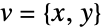
NArgMin[{{1, 1}.v, {{1, 2}, {1, 0}}.v{3, -1}}, v] にスレッディングの可能性があるので,不等式
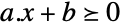 は
 とは等しくないかもしれない:
NArgMin[{{1, 1}.x, {{1, 2}, {1, 0}}.x + {-3, 1}0}, x]NArgMin[{{1, 1}.x, {{1, 2}, {1, 0}}.x{3, -1}}, x] での意図しないスレッディングを避けたければInactive[Plus]を使うとよい:
NArgMin[{{1, 1}.x, {{1, 2}, {1, 0}}.x + {-3, 1}0}, x]定数パラメータを持つ方程式を使って  での意図しないスレッディングを回避する:
parEqs = {a == {{1, 2}, {1, 0}}, b == {3, -1}};NArgMin[{{1, 1}.x, {parEqs, a.x + b0}}, x]VectorGreaterEqualは"NonNegativeCone"についての錐不等式を表す:
constraint = VectorGreaterEqual[{{{1, 2}, {1, 0}}.v, {3, -1}}, "NonNegativeCone"]円錐の次元を明示的に指定したければ,{"NonNegativeCone",n}を使うとよい:
constraint = VectorGreaterEqual[{{{1, 2}, {1, 0}}.v, {3, -1}}, {"NonNegativeCone", 2}]NArgMin[{{1, 1}.v, constraint}, v]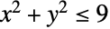

NArgMin[{x + y, x^2 + y^2 ≤ 9}, {x, y}]"NormCone"で錐不等式を使って制約条件 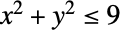 を指定する:
constraint = VectorGreaterEqual[{{x, y, 3}, 0}, {"NormCone", 3}]NArgMin[{x + y, constraint}, {x, y}]

{a, b} = {{{1, 1, 0}, {0, 1, 1}, {1, 1, 1}}, {2, 2, -1}};Indexedを使ってベクトル変数の成分(例: )にアクセスする:
NArgMin[{Total[x], a.xb, Indexed[x, 1] ≥ 1}, x]ベクトル変数の次元と領域が曖昧なときはVectors[n,dom]を使って指定する:
NArgMin[{Indexed[x, {1}] + 2Indexed[x, {2}], (| | |
| --------------- | --------------- |
| Indexed[x, {1}] | 1 |
| 1 | Indexed[x, {2}] |)Underscript[, {"SemidefiniteCone", 2}]0}, x]
NArgMin[{Indexed[x, {1}] + Indexed[2x, {2}], (| | |
| --------------- | --------------- |
| Indexed[x, {1}] | 1 |
| 1 | Indexed[x, {2}] |)Underscript[, {"SemidefiniteCone", 2}]0}, x∈Vectors[2, Reals]]NonNegativeReals ( )を使って非負の制約条件を指定する:
NArgMin[{{1, 1}.x, {Indexed[x, {1}], Indexed[x, {2}], 1}Underscript[, {"NormCone", 3}]0}, x∈Vectors[2, NonNegativeReals]]
NArgMin[{{1, 1}.x, {Indexed[x, {1}], Indexed[x, {2}], 1}Underscript[, {"NormCone", 3}]0, x0}, x]NonPositiveReals ( )を使って非正の制約条件を指定する:
NArgMin[{-Total[v], {1, 2}.v-3}, v∈Vectors[2, NonPositiveReals]]NArgMin[{-Total[v], {1, 2}.v-3, v0}, v]Orによる制約を指定することができる:
NArgMin[{x + y, x ^ 2 + y ^ 2 ≤ 1 || (x + 2) ^ 2 + (y + 2) ^ 2 ≤ 1}, {x, y}]//Quiet領域制約1 (4)
Integersを使って整数領域の制約を指定する:
NArgMin[{x + y, x + 2y ≥ 3, x ≥ -2}, {x, y∈Integers}]Vectors[n,Integers]を使ってベクトル変数に整数領域の制約を指定する:
NArgMin[{Total[x], a == {{1, 2}, {1, 0}}, b == {3, -2},
a.xb}, x∈Vectors[2, Integers]]NonNegativeIntegers ( )を使って非負の整数領域の制約を指定する:
NArgMin[{x + 2y, x^2 + 2y^2 ≤ 3, x + y == 2, x∈NonNegativeIntegers}, {x, y}]NonPositiveIntegers ( )を使って非正の整数領域の制約を指定する:
NArgMin[{-x + y, x + 2y ≥ 3, x∈NonPositiveIntegers}, {x, y}]領域制約2 (5)


t = RotationTransform[{{0, 0, 1}, {1, 1, 1}}];
ℛ = TransformedRegion[Ellipsoid[{0, 0, 0}, {1, 2, 3}], t];NArgMin[z, {x, y, z}∈ℛ]Graphics3D[{{Opacity[0.5], Green, GeometricTransformation[Ellipsoid[{0, 0, 0}, {1, 2, 3}], t]}, {Red, PointSize[Large], Point[%]}}]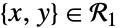
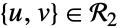
Subscript[ℛ, 1] = Disk[];
Subscript[ℛ, 2] = InfiniteLine[{{-2, 0}, {0, 2}}];NArgMin[EuclideanDistance[{x, y}, {u, v}], {{x, y}∈Subscript[ℛ, 1], {u, v}∈Subscript[ℛ, 2]}]Graphics[{{LightBlue, Subscript[ℛ, 1]}, {Green, Subscript[ℛ, 2]}, {Red, Point[Partition[%, 2]]}}]
Subscript[ℛ, 1] = Triangle[{{0, 0}, {1, 0}, {0, 1}}];
Subscript[ℛ, 2][r_] = Disk[{1, 1}, {2r, r}];NArgMin[{r, {x, y}∈Subscript[ℛ, 1] && {x, y}∈Subscript[ℛ, 2][r]}, {r, x, y}]Graphics[{{LightBlue, Subscript[ℛ, 1], Subscript[ℛ, 2][First[%]]}, {Red, Point[Rest[%]]}}]Subscript[ℛ, 3][{a_, b_, r_}] = Disk[{a, b}, r];NArgMin[{r, ({0, 0} | {1, 0} | {0, 1})∈Subscript[ℛ, 3][{a, b, r}]}, {a, b, r}]Graphics[{{LightBlue, Subscript[ℛ, 3][%]}, {Red, Point[{{0, 0}, {1, 0}, {0, 1}}]}}]Circumsphereを使うと同じ結果が直接得られる:
Circumsphere[{{0, 0}, {1, 0}, {0, 1}}]//N


ℛ = Sphere[];NArgMin[x.{1, 2, 3}, x∈ℛ]線形問題 (5)
線形の目的関数と制約条件がある場合は,最小値が見付かるとそれは大域的になる:
NArgMin[{x + y, 3x + 2y ≥ 7 && x + 2y ≥ 6 && x ≥ 0 && y ≥ 0}, {x, y}]NArgMin[{x - y, x + y + z == 1 / 2, x - 2z == 1, 2x - y ≥ 1}, {x, y, z}]Equalを使っていくつかの等式制約を一度に表現する:
NArgMin[{x - y, {x + y, x - y} == {1 / 2, 1}}, {x, y}]NArgMin[{x - y, x + y == 1 / 2, x - y == 1}, {x, y}]VectorLessEqualを使っていくつかのLessEqual不等式制約を一度に表現する:
NArgMin[{x + y, VectorLessEqual[{{x - 2y, -x + y}, {3, 2}}]}, {x, y}]
 を使ってベクトル不等式をコンパクトな形で入力する:
NArgMin[{x + y, {x - 2y, -x + y}{3, 2}}, {x, y}]NArgMin[{x + y, {x - 2y ≤ 3, -x + y ≤ 2}}, {x, y}]Intervalを使って変数の境界を指定する:
NArgMin[{x + y, x + 2y ≥ 3}, {x∈Interval[{-1, 2}], y∈Interval[{-1, 1}]}]凸問題 (7)
"NonNegativeCone"を使って  の形の線形関数を指定する:
NArgMin[{Total[x],
	VectorGreaterEqual[{{{-1, -1 / 2}, {1, -1 / 2}, {0, 1}}.x, {-1 / 2, -1 / 2, -1 / 2}}, {"NonNegativeCone", 3}]}, x]
 を使ってベクトル不等式をコンパクトな形で入力する:
NArgMin[{Total[x], {{-1, -(1/2)}, {1, -(1/2)}, {0, 1}}.x-(1/2)}, x]NArgMin[{(x - 1)^2 + y^2, x + y / 2 ≤ 1 / 2, x - y ≥ 0}, {x, y}]ContourPlot[(x - 1)^2 + y^2, {x, -1, 1}, {y, -1, 1 / 2}, ...]res = NArgMin[{(x - 1)^2 + y^2, x^2 + (y^2/2) ≤ (1/2), 2x^2 ≤ 3y}, {x, y}]Show[Plot3D[(x - 1)^2 + y^2, {x, -1, 1}, {y, 0, 1}, ...], Graphics3D[{Red, PointSize[0.03], Point[{x, y, (x - 1)^2 + y^2} /. Thread[{x, y} -> res]]}]]

Subscript[ℛ, 1] = Triangle[{{1, 1}, {2, 1}, {1, 2}}];
Subscript[ℛ, 2] = Disk[];NArgMin[EuclideanDistance[x, y], {x∈Subscript[ℛ, 1], y∈Subscript[ℛ, 2]}]Graphics[{{LightBlue, Subscript[ℛ, 1], Subscript[ℛ, 2]}, {Red, Point[%]}}]
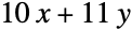
res = NArgMin[{10x + 11 y, (| | |
| - | - |
| x | 1 |
| 1 | y |)Underscript[, {"SemidefiniteCone", 2}]0}, {x, y}]Show[Plot3D[10x + 11y, {x, 0, 5}, {y, 0, 5}, ...], Graphics3D[{Red, PointSize[0.05], Point[{x, y, 10x + 11y} /. Thread[{x, y} -> res]]}]]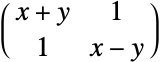

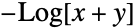
res = NArgMin[{-Log[x + y], (| | |
| ----- | ----- |
| x + y | 1 |
| 1 | x - y |)Underscript[, {"SemidefiniteCone", 2}]0, 1 ≤ x ≤ 10, -1 ≤ y ≤ 1}, {x, y}]Show[Plot3D[-Log[x + y], {x, 1, 10}, {y, -1, 1}, ...], Graphics3D[{Red, PointSize[0.05], Point[{x, y, -Log[x + y]} /. Thread[{x, y} -> res]]}]]res = NArgMin[{(x - 2)^2 + (y - 1 / 2)^2, Inactive[Norm][{x, y}, 4] ≤ 1}, {x, y}]Show[Plot3D[(x - 2)^2 + (y - 1 / 2)^2, {x, -1, 1}, {y, -1, 1}, ...], Graphics3D[{PointSize[0.05], Point[{x, y, (x - 2)^2 + (y - (1/2))^2} /. Thread[{x, y} -> res]]}]]凸に変換可能 (4)
面積1で  の長方形の外周を最小にする高さ
 と重み
 の値を求める:
NArgMin[{2w + 2h, h w == 1, h ≤ (1/2)w, h ≥ 0, w ≥ 0}, {h, w}]この問題は対数凸問題であり,変換{hExp[],wExp[ ]}を行い,対数を取って凸問題を得ることで解ける:
NArgMin[{Log[Exp[𝓌 + Log[2]] + Exp[𝒽 + Log[2]]], 𝒽 + 𝓌 == 0, 𝒽 - 𝓌 ≤ Log[1 / 2]}, {𝒽, 𝓌}]Exp[%]不等式制約とノルム制約に従って擬似凸関数 を最大化する.目的関数は領域上の非負関数と非正関数の積なので,擬似凸関数である:
NArgMin[{-x y, x ≥ 0, y ≥ 0, Norm[{x - 1, y - 2}] ≤ 1}, {x, y}]擬似凸問題はパラメータ  についてのパラメトリック凸最適化問題として解くことができる:
pfun = ParametricConvexOptimization[0, {-x y ≤ α, x ≥ 0, y ≥ 0,
	Norm[{x - 1, y - 2}] ≤ 1}, {x, y}, α, "PrimalMinimizerRules"]
fun[α_ ? NumericQ] := -x * y /. pfun[α];
Plot[fun[α], {α, -4.68, 0}, PlotRange -> All]
pfun[-4.68]pfun[-4.69]
制約条件 に従って
 を最小化する.目的関数は凸ではないが凸関数の差
 として表すことができる.ただし,
 と
 は凸関数である:
res = NArgMin[{x ^ 2 - y ^ 2, Norm[{x, y}] <= 2}, {x, y}]Show[Plot3D[x ^ 2 - y ^ 2, {x, -2, 2}, {y, -2, 2}, ...], Graphics3D[
{PointSize[0.04], Point[{x, y, x ^ 2 - y ^ 2} /. Thread[{x, y} -> res]]}]]制約条件 に従って
 を最小化する.制約条件
 は凸ではないが凸条件の差
 として表すことができる.ただし,
 は凸関数である:
res = NArgMin[{x ^ 2 + y, 1 <= Norm[{x, y}] <= 2}, {x, y}]Show[Plot3D[x ^ 2 + y, {x, -2, 2}, {y, -2, 2}, ...], Graphics3D[
{PointSize[0.04], Point[{x, y, x ^ 2 + y} /. Thread[{x, y} -> res]]}]]一般的な問題 (3)
res = NArgMin[{x + y, Sin[2x] + Cos[3y] ≤ 1, Norm[{x, y}] ≤ 2}, {x, y}]Show[Plot3D[x + y, {x, -2, 2}, {y, -2, 2}, ...], Graphics3D[{Blue, PointSize[0.03], Point[{x, y, x + y} /. Thread[{x, y} -> res]]}]]res = NArgMin[{Sin[2x] + Cos[x], -2 ≤ x ≤ 3}, x]Plot[Sin[2x] + Cos[x], {x, -2, 3}, Epilog -> {PointSize[0.03], Red, Point[{res, Sin[2x] + Cos[x] /. x -> res}]}]非線形目的関数を非線形制約条件に従って最小にする点を求める:
res = NArgMin[{Sin[x^2 + y], Sin[2x] + Cos[3y] ≤ 1, Norm[{x^2, y}] ≤ 2}, {x, y}]Show[Plot3D[Sin[x^2 + y], {x, -2, 2}, {y, -2, 2}, ...], Graphics3D[{Blue, PointSize[0.03], Point[{x, y, Sin[x^2 + y]} /. Thread[{x, y} -> res]]}]]オプション (7)
AccuracyGoalとPrecisionGoal (2)

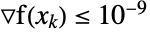
NArgMin[Sin[Tan[x] / 2], x, AccuracyGoal -> 9, PrecisionGoal -> 8]次で,収束基準 と
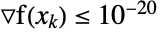 を強制する.これはデフォルトの機械精度計算では達成できない:
NArgMin[Sin[Tan[x] / 2], x, AccuracyGoal -> 20, PrecisionGoal -> 18]
WorkingPrecisionの設定値を高くするとプロセスが収束するようになる:
NArgMin[Sin[Tan[x] / 2], x, AccuracyGoal -> 20, PrecisionGoal -> 18, WorkingPrecision -> 40]EvaluationMonitor (1)
関数の解を求める過程で評価したすべての点を最小値の環で記録する:
f[x_, y_] := (x ^ 2 + y ^ 2 - 16) ^ 2;
{sol, pts} = Reap[
	NArgMin[f[x, y], {{x, -5, 5}, {y, -5, 5}},   Method -> "DifferentialEvolution", EvaluationMonitor :> Sow[{x, y}]]];
訪れた点の中で目的関数の値で最終的な解に近いすべての点をプロットする:
ContourPlot[f[x, y], {x, -5, 5}, {y, -5, 5}, ColorFunction -> (Hue[.6(1 - #1)]&),
	Epilog -> Map[Point, Cases[First[pts], x_ /; Abs[f@@x - f@@sol] ≤ .05]], Contours -> 4Range[0, 10] ^ 2]
Method (2)
メソッドの中には特定の問題に対して準最適化結果を与えるものがある:
objective[x_] := Sin[.4 x ^ 2] + .7Cos[.6 x] x;
NArgMin[{objective[x], -9 < x < 9}, {x}, Method -> #]& /@ {"NelderMead", "DifferentialEvolution", "SimulatedAnnealing"}
この問題の場合は,自動選択されたメソッドが最適な結果を与える:
minSol = NArgMin[{objective[x], -10 < x < 10}, {x}]この非凸問題に対して自動メソッド選択は"Couenne"を選ぶ:
minSol = NArgMin[{objective[x], -10 < x < 10}, {x}, Method -> "Couenne"]Plot[objective[x], {x, -10, 10}, Rule[...]]速度を求めたければ,たくさんの変数がある問題には"NelderMead"メソッドを使う:
n = 50;AbsoluteTiming[NArgMin[Sum[i * (x[i] - i) ^ 2 + Sin[x[i]], {i, 1, n}], Table[x[i], {i, 1, n}], Method -> "NelderMead"]]StepMonitor (1)
NArgMinが古典的なRosenbrock関数の最小値を求めるのに取るステップ:
pts = Reap[NArgMin[(1 - x) ^ 2 + 100(-x ^ 2 - y) ^ 2, {x, y}, Method -> "NelderMead", StepMonitor :> Sow[{x, y}]]][[2, 1]];
pts = Join[{{-1.2, 1}}, pts];ContourPlot[(1 - x) ^ 2 + 100(-x ^ 2 - y) ^ 2, {x, -1.3, 1.5}, {y, -1.5, 1.4}, Epilog -> {Arrow[pts], Point[pts]}, Contours -> Table[10 ^ -i, {i, -2, 10}], ColorFunction -> (Hue[(Log[10, #] + 10) / 12]&), ColorFunctionScaling -> False]WorkingPrecision (1)
作業精度を にする.デフォルトでAccuracyGoalとPrecisionGoalは
 に設定されている:
NArgMin[Cos[x ^ 2 - 3 y] + Sin[x ^ 2 + y ^ 2], {x, y}, WorkingPrecision -> 20]アプリケーション (14)
幾何学の問題 (4)
半径1で中心が 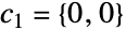 と
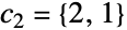 の2つの異なる円板上にある最近点を求める.
 が円板1の上の点,
 が円板2の上の点であるとする.目的は,制約条件に従って
 を最小にすることである:
res = NArgMin[{Norm[p1 - p2], c2 == {2, 1}, Norm[p1] ≤ 1, Norm[p2 - c2] ≤ 1}, {p1∈Vectors[2, Reals], p2∈Vectors[2, Reals]}]Graphics[{{Lighter[Blue], Disk[]}, {Lighter[Red], Disk[{2, 1}]}, {Green, PointSize[0.03], Point[res]}}]

region = [image];

constraints = Table[Norm[Inactive[Plus][pi, -c]] ≤ r, {pi, MeshCoordinates[region]}];res = NArgMin[{r, constraints}, {r, c∈Vectors[3, Reals]}]Show[Graphics3D[{Opacity[0.2], Green, Ball[res[[2]], res[[1]]]}], region]包み込む最小の球はBoundingRegionを使って効率的に求めることができる:
BoundingRegion[region, "MinBall"]3Dの点集合を包み込む, としてパラメータ化される楕円体の体積を最小にする
 と
 の値を求める:
pts = IconizedObject[«With»];

constraints = Table[Norm[a.pi + b] ≤ 1, {pi, pts}];
res = NArgMin[{-Log[Det[a]], constraints, aUnderscript[, {"SemidefiniteCone", 3}]0}, {a, b∈Vectors[3]}]
{Σ, x0} = {Inverse[Transpose[res[[1]]].res[[1]]], -LinearSolve[res[[1]], res[[2]]]};
minVolEllipsoid = Ellipsoid[x0, Σ]Graphics3D[{{Opacity[0.3], Red, Ellipsoid[x0, Σ]}, {PointSize[0.025], Point[pts]}}]境界楕円体の体積は,最小であるとは限らないが,BoundingRegionで求めることもできる:
fastEllipsoid = BoundingRegion[pts, "FastEllipsoid"]{Volume[minVolEllipsoid], Volume[fastEllipsoid]}指定された半径  (
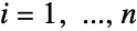 )で重なり合ない
 個の円を収めることができる最小の正方形を求める.円の数と各円の半径を指定する:
n = 3;
r = BlockRandom[RandomReal[{0.5, 1.5}, n], RandomSeeding -> 123]; が円
 の中心なら,目的は
 を最小化することである.
 を最小にして
 とするために目的を変形することができる:
objectiveConstraint = Table[-s <= Norm[c[i], Infinity] + r[[i]] <= s, {i, n}];nonOverlapConstraint = Table[Norm[c[i] - c[j]] >= r[[i]] + r[[j]],
{i, 1, n}, {j, i + 1, n}];vars = Append[Table[Element[c[i], Vectors[2, Reals]], {i, n}], Element[s, Reals]];円は正方形 の中に収まっている.境界ボックスと各円の中心を求める:
res = NArgMin[{s, objectiveConstraint, nonOverlapConstraint}, vars, Method -> "DifferenceOfConvex"]Graphics[{Table[Circle[res[[i]], r[[i]]], {i, n}], {FaceForm[None], EdgeForm[Thickness[Medium]], Rectangle[{-res[[-1]], -res[[-1]]}, {res[[-1]], res[[-1]]}]}}]Sum[Area[Disk[res[[i]], r[[i]]]], {i, n}] / Area[Rectangle[{-res[[-1]], -res[[-1]]}, {res[[-1]], res[[-1]]}]]データフィッティング問題 (3)
与えられた行列 a とベクトル b について,制約条件  に従って
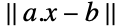 を最小化する点を求める:
{a, b} = IconizedObject[«Block»];NArgMin[{Norm[Inactive[Plus][a.x, -b]], x1}, x]データの最初と最後の点が曲線上にあるようにして,三次曲線を離散データにフィットする:
data = IconizedObject[«Block»];DesignMatrixを使って行列を構築する:
a = DesignMatrix[data, {1, x, x^2, x^3}, x];
b = data[[All, 2]];
最初と最後の点が曲線上になければならないという制約条件を定義する:
pointConstraints = {a[[1]].λ == b[[1]], a[[-1]].λ == b[[-1]]};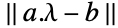

res = NArgMin[{Norm[Inactive[Plus][a.λ, -b]], pointConstraints}, λ]Show[Plot[Evaluate[{1, x, x^2, x^3}.res], {x, 0, 1}, Epilog -> {Red, PointSize[0.03], Point[data[[{1, -1}]]]}], ListPlot[data]]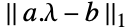 を最小にする
 の値を求めることで,外れ値にあまり敏感ではない非線形離散データのフィットを求める:
data = IconizedObject[«Block»];

bases = Sqrt[1 + (x - #) ^ 2]& /@ Subdivide[-3, 3, 10];
input = DesignMatrix[data, bases, x, IncludeConstantBasis -> False];
output = data[[All, 2]];res = NArgMin[{Norm[Inactive[Plus][a.λ, -b], 1], a == input, b == output}, λ]Plot[Evaluate[bases.res], {x, -3, 3}, Epilog -> {PointSize[0.008], Point[data]}]Plot[{Sin[2x] + Cos[x ^ 2], Evaluate[bases.res]}, {x, -3, 3}, PlotLegends -> {"Reference", "SubscriptBox[L, 1]fit"}]分類問題 (3)



{set1, set2} = IconizedObject[«Block»];分離するためには,集合1は 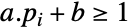 を,集合2は
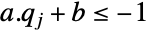 を満足しなければならない:
constraints = {set1.a + b1, set2.a + b-1};目的は を最小にすることだが,そうすると
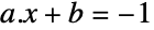 と
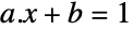 の間の厚みの2倍が与えられる:
res = NArgMin[{Norm[a], constraints}, {a, b}]line = res[[1]].{x, y} + res[[2]]Show[RegionPlot[line ≤ 0, {x, 0, 1}, {y, 0, 1}], ListPlot[{set1, set2}, PlotMarkers -> {Automatic, PointSize[0.025]}]]

{set1, set2} = IconizedObject[«Block»];
dataplot = ListPointPlot3D[{set1, set2}, Sequence[...]]DesignMatrixを使って2つの集合のための二次多項式データ行列を構築する:
{data1, data2} = DesignMatrix[#, {x, x^2, y, y^2, x y}, {x, y}]& /@ {set1, set2};分離するためには,集合1は 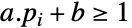 を,集合2は
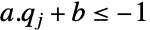 を満足しなければならない:
constraints = {data1.a + b1, data2.a + b-1};
res = NArgMin[{Norm[a], constraints}, {a, b}, PrecisionGoal -> 3]poly = (res[[1]].{1, x, x^2, y, y^2, x y} + res[[2]])Show[dataplot, ContourPlot3D[poly == 0, {x, -1.5, 1.5}, {y, -1.5, 1.5}, {z, -1, 1}, Sequence[...]]]与えられた点集合  を異なる集合に分割する.これは,
 を最小にすることで各集合の中心
 を求めることで行える.ただし,
 は与えられた局所カーネルで
 は与えられたペナルティパラメータである:
x = IconizedObject[«Block»];
{n, dim} = Dimensions[x];
centers = Indexed[μ, #]& /@ Range[n];
カーネル  は,もし
 ならば
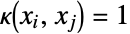 ,それ以外では
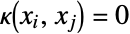 の
 最近傍(
 )関数である.この問題のために
 最近傍が選ばれた:
kNN = Nearest[x -> Automatic][x, 10];
κ = SparseArray[Join@@Table[Thread[{i, kNN[[i]]}], {i, n}] -> 1, {n, n}];
c1 = Table[Norm[Inactive[Plus][Indexed[x, {i}], -Indexed[μ, {i}]]], {i, n}];
c2 = Flatten[Table[κ[[i, j]]Norm[Indexed[μ, {i}] - Indexed[μ, {j}], 1], {i, 1, n}, {j, i + 1, n}]];
objective = Total[c1 ^ 2] / 2 + 10 Total[c2];vars = Table[Indexed[μ, {i}]∈Vectors[dim, Reals], {i, n}];res = NArgMin[objective, vars];各データ点に対応する中心が存在する.同じ集合に属するデータは同じ中心を持つ:
allCenters = res;
cvals = Map[First, Gather[allCenters, Norm[#1 - #2] ≤ 0.001&]]gpts = Table[Pick[x, Map[Norm[# - ci] ≤ 0.001&, allCenters]], {ci, cvals}];
Show[ListPlot[gpts, PlotStyle -> PointSize[0.02]], ListPlot[allCenters, PlotStyle -> {PointSize[0.03], Magenta}]]画像処理 (1)
全変動ノルムの下で最も近い画像を求めることで,破損した画像を回復する:
image = ImageResize[ColorConvert[ExampleData[{"TestImage", "House"}], "Grayscale"], 75]40%のデータ点をランダムに削除することで破損画像を作成する:
data = ImageData[image];
SeedRandom[123];
mask = RandomChoice[{0.4, 0.6} -> {0, 1}, Dimensions[data]];
corruptedData = mask * data;
Image[corruptedData]
目的は を最小にすることである.ただし,
 は画像データである:
{n, m} = Dimensions[data];objective = Total[Flatten[Table[Norm[{Indexed[u, {i + 1, j}] - Indexed[u, {i, j}], Indexed[u, {i, j + 1}] - Indexed[u, {i, j}]}], {i, n - 1}, {j, m - 1}]]];任意の非零のデータ点  は破損していないと仮定する.これらの点について,
 と設定する:
knownPos = SparseArray[mask]["NonzeroPositions"];constraint = Map[Indexed[u, #] == data[[Sequence@@#]]&, knownPos];sol = NArgMin[{objective, constraint}, u∈Matrices[{n, m}, Reals]];Image[sol]施設の場所の問題 (1)
さまざまな携帯電話基地局  の場所と
 にいるクライアントにサービスを提供するために必要な範囲
 を求める:
clientPos = {{0, 0}, {1, 0}, {3 / 2, 1}, {-1 / 2, 1}, {1 / 2, 3 / 2}, {1 / 2, 1 / 2}, {0, 3 / 2}, {1, 1}, {0, 1}, {3 / 2, 3 / 2}};
nTowers = 3;
nClients = Length[clientPos];
各基地局は,範囲に比例する電力( で与えられる)を消費する.目的は電力消費量を最小にすることである:
objective = Sum[Erf[r[i] ^ 1.5], {i, nTowers}]; を,クライアント
 が携帯基地局
 でカバーされるなら
 であることを示す決定変数とする:
decisionConstraint = 0z1;各携帯基地局はその範囲がクライアントの何人かをカバーするような場所になければならない:
m = 20;
distConstraint = Table[Norm[{p[j, 1], p[j, 2]} - clientPos[[i]]] -
m * (1 - Indexed[z, {i, j}]) ≤ r[j], {i, nClients}, {j, nTowers}];coverageConstraint = Total[z, {2}]1;maxCoverageConstraint = Table[0 ≤ r[j] ≤ 1, {j, nTowers}];vars = Flatten[{Table[{p[j, 1], p[j, 2], r[j]}, {j, nTowers}], z∈Matrices[{nClients, nTowers}, Integers]}];Quiet[res = NArgMin[{objective, decisionConstraint,
distConstraint, coverageConstraint, maxCoverageConstraint}, vars]]towerPos = Table[{p[i, 1], p[i, 2]}, {i, nTowers}] /. Thread[vars -> res]
towerRange = Table[r[i], {i, nTowers}] /. Thread[vars -> res]各携帯基地局の位置とその範囲をクライアントの場所について可視化する:
Graphics[{{StandardYellow, PointSize[0.04], Point[towerPos]}, {StandardBlue, PointSize[0.02], Point[clientPos]}, {...}}, Frame -> True]ポートフォリオの最適化 (1)
リスクが最小でリターンか最大になるような,資本  の6つの株式への投資配分を求める:
{μ, Σ} = Block[...];リターンは  で与えられる.ただし,
 は個別の株式の予想収益の値のベクトルである:
return = μ.w;リスクは  で与えられる.
 はリスク回避パラメータであり,
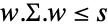 である:
risk = w.Σ.w;
riskConstraint = risk ≤ s;
目的は,指定されたリスク回避パラメータについてリスクを最小にしつつリターンを最大にすることである:
objective[α_ ? NumericQ] := -(return - α s);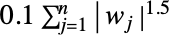
marketConstraints = Table[Abs[Indexed[w, i]] ^ 1.5 ≤ Indexed[t, i], {i, 6}];重み  はどれも0より大きくなければならず,重みに市場影響コストを加えたものは1でなければならない:
weightConstraints = {w0, Total[w] + 0.1Total[t] == 1};リスク回避パラメータの範囲について,利益と対応するリスクを計算する:
frontier = Table[res = Quiet@NArgMin[{objective[α],
	riskConstraint, weightConstraints, marketConstraints}, {w, s, t∈Vectors[6, Reals]}];
	{risk, return} /. w -> res[[1]], {α, Subdivide[0, 10, 100]}];
範囲  での最適な
 は,リスクとリターンのトレードオフの上界包絡線を与える:
randomRiskReturns = Table[{risk, return}, {w, Table[...]}];
Show[ListPlot[frontier, ...], ListPlot[randomRiskReturns, Rule[...]]]riskAversionParameter = N@{1 / 1000, 1 / 100, 1 / 2, 1, 5, 10, 15, 20};
res = Table[{α, return, Quiet@Append[w, 1 - Total[w]]} /.
w -> Quiet@NArgMin[{objective[α],
riskConstraint, weightConstraints, marketConstraints}, {w, s, t∈Vectors[6, Reals]}][[1]], {α, riskAversionParameter}];市場コストを説明することで,低リスク回避のための多様化したポートフォリオが得られるが,リスク回避が高い場合は,多様化されていない株式を購入するため,市場への影響コストが支配的になる:
Legended[BarChart[res[[All, -1]], ...], SwatchLegend[...]]軌道の最適化 (1)
始点と終点の間の距離が最短となるような円形障害物を避ける経路を求める:
p = {{2, 2}, {7, 6}, {3, 5}, {4, 8}, {8, 9}, {6, 2.5}};
r = {1, 1.3, 1.5, 1, 0.7, 1.5};
{start, end} = {{0, 0}, {10, 10}};
domain = Graphics[{MapThread[Circle[#1, #2]&, {p, r}],
	{PointSize[0.02], Point[{start, end}]}}, Frame -> True]
経路は  個の異なる点に離散化できる.点と点の間の距離は
 未満でなければならない.ただし,
 は最短とする距離である:
n = 30;
distanceConstraints = Table[Inactive[Norm][x[i] - x[i - 1]] <= l / n, {i, n}];objectConstraints = Table[Inactive[Norm][-p[[j]] + x[i]] >= r[[j]], {i, 1, n}, {j, 1, 6}];positionConstraints = {x[0] == start, x[n] == end};vars = Append[Table[x[i]∈Vectors[2, Reals], {i, 0, n}], l∈Reals];
Short[res = NArgMin[{l, distanceConstraints, objectConstraints,
positionConstraints}, vars, Method -> "DifferenceOfConvex"], 4]Show[domain, Graphics[{Red, Point[res[[1 ;; -2]]]}]]特性と関係 (6)
NMinimizeは最小値と,変数の値を最小にする規則を与える:
NMinimize[{x.x + y, Norm[x + y] ≤ 1}, {Element[x, Vectors[2, Reals]], y}]NArgMinは最小にする値のリストを与える:
NArgMin[{x.x + y, Norm[x + y] ≤ 1}, {Element[x, Vectors[2, Reals]], y}]NMinValueは最小値だけを与える:
NMinValue[{x.x + y, Norm[x + y] ≤ 1}, {Element[x, Vectors[2, Reals]], y}]NArgMin[{x ^ 2 + y ^ 2, x + 2 y ≥ 3}, {x, y}]NArgMax[{-(x ^ 2 + y ^ 2), x + 2 y ≥ 3}, {x, y}]凸問題については,ConvexOptimizationを使って追加的な解の特性が得られるかもしれない:
NArgMin[{x ^ 2 + y ^ 2, x + 2 y ≥ 3}, {x, y}]ConvexOptimization[x ^ 2 + y ^ 2, x + 2 y ≥ 3, {x, y}, "PrimalMinimizer"]ConvexOptimization[x ^ 2 + y ^ 2, x + 2 y ≥ 3, {x, y}, "DualMaximizer"]パラメータがある凸問題について,ParametricConvexOptimizationを使うとParametricFunctionが与えられる:
pfun = ParametricConvexOptimization[x + 2 y, (x - α) ^ 2 + (y - β) ^ 2 ≤ 1, {x, y}, {α, β}, "PrimalMinimizer"]ParametricFunctionはパラメータの値について評価できる:
{pfun[0., 0.], pfun[.5, 1.], pfun[2., 1.]}NArgMinを使ってパラメトリック問題についての関数を定義する:
fun[α_ ? NumericQ, β_ ? NumericQ]  := NArgMin[{x + 2 y, (x - α) ^ 2 + (y - β) ^ 2 ≤ 1}, {x, y}];
{fun[0., 0.], fun[.5, 1.], fun[2., 1.]}testData = RandomReal[{0, 4}, {1000, 2}];
{First[AbsoluteTiming[pfun @@@testData]], First[AbsoluteTiming[fun @@@ testData]]}ParametricFunctionの導関数も計算できる:
D[pfun[α, β], {{α, β}}] /. {α -> 2., β -> 1.}RobustConvexOptimizationは,パラメータ制約がある凸問題についてはパラメータの可能なすべての値について有効な最適値を求める:
{rMinValue, rMin} = RobustConvexOptimization[2x + 3y, x + y ≥ α && x - y ≤ β && -1 ≤ α ≤ 1 && 0 ≤ β ≤ 1, {x, y}, {α, β}, {"PrimalMinimumValue", "PrimalMinimizerRules"}]NArgMinはパラメータの特定の値についてより小さい最小値を与えるミニマイザを求めるかもしれない:
minimizer0 = NArgMin[{2x + 3y, x + y ≥ α && x - y ≤ β && α == 0 && β == 0}, {x, y}]Function[{x, y}, 2x + 3 y]@@ minimizer0このミニマイザは  と
 の使用可能なすべての値についての制約条件は満足しない:
(Function[{x, y}, x + y ≥ α && x - y ≤ β ]@@ minimizer0) /. {α -> 1, β -> 1}パラメータの特定の値について求まった最小値はロバストな最小値以下である:
fun[α_, β_] /; (-1 ≤ α ≤ 1 && 0 ≤ β ≤ 1)  :=
NMinValue[{2x + 3y, x + y ≥ α && x - y ≤ β}, {x, y}];testValues = RandomVariate[UniformDistribution[{{-1, 1}, {0, 1}}], 100];
AllTrue[testValues, ((fun@@#) ≤ rMinValue)&]RegionNearestを使って指定された領域の最近点を計算する:
ℛ = Cone[{{-1, 0, 1}, {2, 3, 4}}, 3];
p = {3., 2., 1.};RegionNearest[ℛ, p]//RootReduceこれは,NArgMinを使っても計算できる:
NArgMin[Norm[{x, y, z} - p], {x, y, z}∈ℛ]Graphics3D[{ℛ, {PointSize[Large], {Green, Point[p]}, {Red, Point[%]}}}]

テキスト
Wolfram Research (2008), NArgMin, Wolfram言語関数, https://reference.wolfram.com/language/ref/NArgMin.html (2024年に更新).
CMS
Wolfram Language. 2008. "NArgMin." Wolfram Language & System Documentation Center. Wolfram Research. Last Modified 2024. https://reference.wolfram.com/language/ref/NArgMin.html.
APA
Wolfram Language. (2008). NArgMin. Wolfram Language & System Documentation Center. Retrieved from https://reference.wolfram.com/language/ref/NArgMin.html