



Reduce
詳細とオプション
- 命題 expr は次の論理結合のいずれでもよい.
-
lhs==rhs 等しい lhs!=rhs 等しくない lhs>rhs または lhs>=rhs 不等式 expr∈dom 定義域指定 {x,y,…}∈reg 値域指定 ForAll[x,cond,expr] 全称記号 Exists[x,cond,expr] 存在記号 - Reduce[expr,vars]の結果は常に expr と全く等しい数学的な集合を表す.
- Reduce[{expr1,expr2,…},vars]はReduce[expr1&&expr2&&…,vars]と等価である.
- Reduce[expr,vars]は,デフォルトで,不等式に代数的に現れる限定子は実数で,その他の限定子は複素数であると仮定する.
- Reduce[expr,vars,dom]は,すべての変数とパラメータを定義域 dom に属するものに限る.
- dom がRealsであるか,あるいはIntegersやRationalsのような部分集合の場合,すべての定数と関数の値もまた実数に限られる.
- Reduce[expr&&vars∈Reals,vars,Complexes]は実数と仮定される変数の簡約を行うが,関数の値は複素数であっても構わない.
- Reduce[expr,vars,Integers]は整数についてディオファントス(Diophantus)方程式を簡約する.
- Reduce[…,x∈reg,Reals]は,x が値域 reg になるように制限する.x の異なる座標にはIndexed[x,i]を使って言及することができる.
- Reduce[expr,{x1,x2,…},…]は,実質的に expr を x1, x2, …に対する制約条件の論理結合として表現する.ただし各条件は直前の
 のみが関連するものとする.
 - expr 中の
 を含まない代数的変数は独立パラメータとして扱われる.
 - Reduce[expr,…]の結果にLogicalExpandを適用すると,
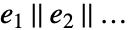 という形式の式が与えられる.ただし,各
  は expr が定義する集合中の個々の構成要素であると考えられる.
  は解体してはならないが,異なる次元を持つことはできる.LogicalExpandの後,各
  は
は  という形式になる.
- LogicalExpandがなければ,Reduceはデフォルトで
 の条件をネストしたものを連続したレベルでOrとAndを交互に組み合せて返す.
 - expr が実数あるいは複素数の定義域の整方程式と不等式のみを含む場合は,Reduceは原則的に常にすべての
 について直接解くことができる.
 - expr が超越条件や整数の定義域を含んでいる場合,Reduceはしばしば結果に付加的なパラメータを導入する.
- expr が多項式条件のみを含む場合,Reduce[expr,vars,Reals]は expr の柱状代数分解(CAD)を与える.
- Reduceは整数についてのすべての線形方程式と不等式の明示的な解の表示を与えることができ,文献中のディオファントス方程式の大部分を解くことができる.
- expr が実数または複素数の定義域で多項式条件のみを含む場合,Reduce[expr,vars]は結果に数量的変数が含まれないように常に限定子を除去する.
- 指定可能なオプション
-
Backsubstitution False 逆置換によってほどいた結果を与えるか否か » Cubics False すべての三次関数を解くために明示的な根号を使うか否か » GeneratedParameters C 生成したパラメータの命名法 » Modulus 0 整数に仮定するモジュール » Quartics False 四次方程式を解くために明示的な根号を使うか否か » - Reduce[expr,{x1,x2,…},Backsubstitution->True]は,特定の
 の条件が以前の
  に最低限しか依存しないように,
 のために以前に生成された方程式の値が逆置換された形を与える. »
例題
すべて開く すべて閉じる例 (4)
Reduce[x ^ 2 - y ^ 3 == 1, {x, y}]Reduce[x ^ 2 + y ^ 2 < 1, {x, y}]Reduce[x ^ 2 - 7y ^ 2 == 1 && x > 0 && y > 0, {x, y}, Integers]Reduce[x ^ 2 - 7y ^ 2 == 1 && x > 0 && y > 0, {x, y}, Reals]Reduce[Exists[{x, y}, x ^ 2 + a y ^ 2 ≤ 1 && x - y ≥ 2], a]Reduce[{x, y}∈InfiniteLine[{{0, 0}, {2, 2}}] && {x, y}∈Circle[], {x, y}]Graphics[{Blue, Circle[], InfiniteLine[{{0, 0}, {2, 2}}], {Red, Point[{x, y}] //. {ToRules[%]}}}]スコープ (83)
基本的な用法 (5)
Reduce[x ^ 2 + y ^ 2 == 2 && x - y == 1, {x, y}]ToRulesおよびReplaceRepeated (//.)を使って解をリストにする:
{x, y} //. {ToRules[%]}Reduce[x ^ 2 + y ^ 2 < 2 && x - y ≥ 1, {x, y}]Reduce[(x ^ 4 - 1)(x ^ 4 - 4) == 0, x, Complexes]Reduce[(x ^ 4 - 1)(x ^ 4 - 4) == 0, x, Reals]Reduce[(x ^ 4 - 1)(x ^ 4 - 4) == 0, x, Integers]Reduce[a x ^ 2 + b x + c == 0, x]解を表すためには新たなパラメータを導入する必要があるかもしれない:
Reduce[Sin[x] == 1 / 2, x]Reduce[x ^ 2 - 2y ^ 2 == 1 && x > 0 && y > 0, {x, y}, Integers]% /. Table[{C[1] -> i}, {i, 10}]//Simplify複素領域 (16)
Reduce[2 x + 3y - 5z == 1 && 3x - 4y + 7z == 3, {x, y, z}]Reduce[x ^ 3 - 2x + 1 == 0, x]Reduce[x ^ 2 - y z == 1, {x, y, z}]Reduce[x ^ 2 + y ^ 3 == z && x + 2y == 3z + 1 && x y z ≠ 0, {x, y, z}]Reduce[ForAll[x, Exists[y, a x ^ 2 + b y ^ 2 - 3y == 1 && y ≠ 0]], {a, b}]Reduce[Sqrt[x + 2y] - 3x + 4y == 5 && x + y ^ (1 / 3) == 1, {x, y}]Reduce[Sin[x] == 1 / 3, x]Reduce[ 4 ^ (x ^ 2)2 ^ x == 8, x]Reduce[Log[x] == 75 / 11 I Pi + 17, x]Reduce[JacobiSN[x, y] == 1, x]Reduce[Zeta[x] == 0, x]
Reduce[Zeta[x] == 0 && Re[x] == 1 / 2 && Im[x] ^ 2 < 500, x]Reduce[Sin[E ^ x] - Cos[2 x] == 1 && -1 ≤ Re[x] ≤ 1 && -1 ≤ Im[x] ≤ 1, x]Reduce[Gamma[x] - Log[x] == I / 2 && Abs[x - 2] < 3 / 2, x]以下ではReduceがある種の解を求めたが,他の解がないことは証明できない:
Reduce[x == E ^ (1 / x) && Abs[x] < 5, x]
Reduce[Cos[Exp[x]] == 3 Exp[-x] + 1 && 0 ≤ Re[x] ≤ 1, x]Reduce[JacobiCS[x, 3] == 1 + I, x]Reduce[Sin[x + y] == 1 / 2 && E ^ x - y == 1, {x, y}]Reduce[FresnelS[x - y] - AiryAi[x] + y == (3 + I) / 2 && CosIntegral[x] y - Sin[x y] == -5(1 - I) / 4 && 1 ≤ Re[x] ≤ 2 && 0 ≤ Im[x] ≤ 1 && 1 ≤ Re[y] ≤ 2 && 0 ≤ Im[y] ≤ 1, {x, y}]実領域 (26)
Reduce[2 x + 3y - 5z == 1 && 3x - 4y + 7z == 3, {x, y, z}, Reals]Reduce[x ^ 5 - 2x + 1 == 0, x, Reals]Reduce[x ^ 5 - 2x + 1 < 0, x, Reals]Reduce[x ^ 2 - y z == 1, {x, y, z}, Reals]Reduce[x ^ 2 - 2y + z ^ 2 ≤ 1, {x, y, z}, Reals]Reduce[x ^ 2 + y z == 1 && x + 2y ≤ 3z + 1 && x y z > 7, {x, y, z}, Reals]Reduce[ForAll[x, Exists[y, a x ^ 2 + b y ^ 2 - 3y == 1 && y < 0]], {a, b}, Reals]Reduce[Sqrt[x + 2y] - 3x + 4y ≥ 5 && x + y ^ (1 / 3) == 1, {x, y}, Reals]Reduce[Abs[(x + Abs[x + 2]) ^ 2 - 1] ^ 2 == 9, x, Reals]Reduce[Max[x, y] == Min[y ^ 2 - x, x], {x, y}]Reduce[Abs[3x ^ 2 - 7x - 6] < Abs[x ^ 2 + x], x, Reals]Reduce[Floor[x ^ 2 + Ceiling[x ^ 2]] < 10, x, Reals]Reduce[E ^ x - x == 7, x, Reals]Reduce[ 27^2x - 1^(1/(x)) == Sqrt[9^2x - 1], x, Reals]Reduce[Sin[x] < 1 / 3, x, Reals]Reduce[ (1/2^x - 1) > (1/1 - 2^x - 1), x, Reals]Reduce[1 < JacobiNC[x, 3] ≤ 2, x, Reals]Reduce[AiryBi[1 - x ^ 2] == 0 && 99 < x < 100, x, Reals]Reduce[900 < AiryAiZero[2t + 1] ^ 2 < 1000, t, Reals]Reduce[E ^ (2E ^ x) - Log[x ^ 2 + 1] - 20x == 11, x, Reals]Reduce[x ^ 1000000 - 2x ^ 777777 + 3x ^ 12345 + 9x ^ 67 - 10 == 0, x, Reals]Reduce[2x ^ (123451 / 67890) - x ^ 2 + 4Sqrt[x] - 4x - 9 / 8 == 0, x, Reals]Reduce[x ^ Pi - x ^ x ^ Sqrt[2] - Sqrt[3]x + 2 ^ (1 / 3) == 0, x, Reals]Reduce[E ^ (2E ^ x) - Log[x ^ 2 + 1] - 20x < 11, x, Reals]Reduce[2Sin[Exp[x]] - Cos[Pi x] == 3 / 2 && -1 < x < 1, x, Reals]Reduce[Cos[x] - BesselJ[5, x] == 1 / 2 && 0 ≤ x ≤ 10, x]Reduce[Gamma[x] ≤ 2x && -2 ≤ x ≤ 2, x, Reals]
Reduce[Exp[Sin[x]] - Sin[3 Cos[x]] == 0, x, Reals]Reduce[Sin[x + y] == 1 / 2 && E ^ x - y ≤ 1, {x, y}, Reals]Reduce[ 3^x - 2^2y == 77 && Sqrt[3^x] - 2^y == 7, {x, y}, Reals]Reduce[E ^ x y ^ 3 + Log[x]y == 1 && x y + E ^ x / x ≥ 2, {x, y}, Reals]Reduce[E ^ x y ^ 3 + Log[x] y > 3x, {x, y}, Reals]Reduce[Exists[a, a x ^ 2 + Sinh[x ^ 2 + 1]a ^ 2 ≥ 1 && x ^ 2 + a ^ 2 ≤ 1], x, Reals]Reduce[Sin[x - Cos[x]] y ^ 3 - x == 1 && x ^ 2 + y ^ 2 ≤ 1, {x, y}, Reals]Reduce[Exists[y, y ^ 3 - Cos[x] y + 2 x ^ 2 Sin[x ^ 2 - 1] > 0 && x ^ 2 + Cos[x] ^ 2 ≤ 2], x, Reals]Reduce[y ^ 3 - BesselJ[2, x + 2] y - y - 3 x == -2 && y < 0 && x ^ 2 < 2, {x, y}, Reals]Reduce[Exists[y, y ^ 4 - Gamma[x + 2] y - y - 3 ArcSin[x / 3] == 1 && y < -1 / 2 && 0 < x < 2], x, Reals]Reduce[Gamma[x + y + 1] - Sin[x y] == 1 && Erf[x ^ 2 - y] - E ^ y - x + 4 == 0 && 0 < x < 3 && 0 < y < 3, {x, y}, Reals]整数領域 (13)
Reduce[2 x + 3y - 5z == 1 && 3x - 4y + 7z == 3, {x, y, z}, Integers]Reduce[2 x + 3y == 4 && 3x - 4y ≤ 5 && x - 2y > -21, {x, y, z}, Integers]Reduce[x ^ 1000 - 2x ^ 777 + 1 == 0, x, Integers]Reduce[x ^ 5 - 2x + 1 < 0, x, Integers]Reduce[x ^ 2 + x y + y ^ 2 == 109, {x, y}, Integers]Reduce[x ^ 2 - 3y ^ 2 == 22 && x > 0 && y > 0, {x, y}, Integers]Reduce[x ^ 2 - 6 x y + 9y ^ 2 - x + 2y == 1, {x, y}, Integers]Reduce[x ^ 3 - 2x ^ 2 y + y ^ 3 == 2, {x, y}, Integers]Reduce[x ^ 2 + 4y ^ 2 + 9z ^ 2 + 16t ^ 2 == 354 && x > 0 && y > 0 && z > 0 && t > 0, {x, y, z, t}, Integers]Reduce[x ^ 2 + y ^ 2 == z ^ 2, {x, y, z}, Integers]Reduce[x ^ 4 + y ^ 4 + z ^ 4 ≤ 500 && x + y ^ 2 + z ^ 3 == 32, {x, y, z}, Integers]Reduce[2x ^ 7 + 8y ^ 15 + 14 x y z == 3, {x, y, z}, Integers]Reduce[Exp[y ^ 2] < x && Abs[x] < 5 && Abs[y] < 5, {x, y}, Integers]Reduce[Exp[x ^ 2 - 5y ^ 2 + 1] + x ^ 2 - 5y ^ 2 == 0 && x > 0 && y > 0, {x, y}, Integers]Reduce[Mod[x ^ 2 + y ^ 2, 2] == 1 && Mod[x - 2y, 3] == 2, {x, y}, Integers]Reduce[GoldenRatio x ^ 2 - Sqrt[5] y ^ 2 - z == Sqrt[5], {x, y, z}, PositiveIntegers]Reduce[Pi x ^ 2 + Sqrt[6]x y - Sqrt[3] y ^ 3 + Pi ^ 2 Sqrt[3] y ^ 2z ^ 2 - 3Sqrt[3] y z == Sqrt[2(109 + 12Sqrt[3])] + 4Pi + 144Sqrt[3]Pi ^ 2 - Sqrt[2] - 63 Sqrt[3], {x, y, z}, Integers]モジュラ領域 (5)
Reduce[2 x + 3y - 5z == 1 && 3x - 4y + 7z == 3, {x, y, z}, Modulus -> 12]Reduce[x ^ 3 - 2x + 1 == 0, x, Modulus -> 5]Reduce[x ^ 2 - y z == 1, {x, y, z}, Modulus -> 4]Reduce[x ^ 2 + y ^ 3 == z && x + 2y == 3z + 1 && x y z ≠ 0, {x, y, z}, Modulus -> 7]Reduce[ForAll[x, Exists[y, a x ^ 2 + b y ^ 2 - 3y == 1 && y ≠ 0]], {a, b}, Modulus -> 3]有限体領域 (4)
ℱ = FiniteField[53, 4];
Reduce[x ^ 5 + ℱ[123]x == ℱ[234], x]Reduce[x ^ 7 + 2 x + 3 == 0, x, ℱ]ℱ = FiniteField[71, 2];
Reduce[ℱ[123]x + ℱ[234]y == ℱ[345] && ℱ[321]x + ℱ[432]y == ℱ[543], {x, y}]Reduce[ℱ[1234]x + ℱ[2345]y + ℱ[3456]z == ℱ[4567] && ℱ[1]x + ℱ[2]y + ℱ[3]z == ℱ[4], {x, y, z}]ℱ = FiniteField[7, 5];
Reduce[x ^ 2 + y ^ 2 == 3 && x ^ 5 + y ^ 5 == 5, {x, y}, ℱ]Reduce[ℱ[123]x ^ 2 + ℱ[234]y ^ 3 + ℱ[345]z ^ 4 == ℱ[456] && ℱ[21]x + ℱ[32]y ^ 2 + ℱ[43]z ^ 3 == ℱ[54] && x y z == ℱ[1], {x, y, z}]ℱ = FiniteField[2, 5];
Reduce[Exists[z, ℱ[1]x + ℱ[3]y + ℱ[5]z == ℱ[7] && ℱ[21]x + ℱ[23]y + ℱ[25]z == ℱ[27]], {x, y}]Reduce[Exists[{y, z}, ℱ[1]x ^ 2 + ℱ[2]y ^ 3 + ℱ[3]z ^ 4 == ℱ[4] && ℱ[5]x ^ 4 + ℱ[6]y ^ 3 + ℱ[7]z ^ 2 == ℱ[8] && x y z != ℱ[0]], x]混合領域 (4)
Reduce[x ^ 2 + y ^ 2 == 1 && Element[x, Reals], {x, y}] が実数で
が実数で より小さい場合について,
 の実数値と
の実数値と  の複素数値を求める:
Reduce[x ^ 2 + y ^ 2 < 1 && Element[x, Reals], {x, y}, Complexes]Abs[x]を含む不等式を簡約する:
Reduce[1 < Abs[ (z - 2/2z - 1)] < 2, z]Block[{z = u + I v}, RegionPlot[1 < Abs[ (z - 2/2z - 1)] < 2, {u, -1, 1}, {v, -1, 1}]]Reduce[x ^ 2 + y ^ 2 < 5 && Element[x, Integers], {x, y}, Reals]幾何学領域 (10)
Subscript[ℛ, 1] = Circle[];
Subscript[ℛ, 2] = Line[{{-2, 1}, {1, -2}}];Reduce[{x, y}∈Subscript[ℛ, 1] && {x, y}∈Subscript[ℛ, 2], {x, y}]Graphics[{{Blue, Subscript[ℛ, 1], Subscript[ℛ, 2]}, {Red, Point[{x, y}] //. {ToRules[%]}}}]Reduce[2 x + 3 y - 5 z == 1 && 2 x y == z^2 && {x, y, z}∈Sphere[], {x, y, z}, Reals]Show[{ContourPlot3D[{2 x + 3 y - 5 z == 1, 2 x y == z^2}, {x, -1.2, 1.2}, {y, -1.2, 1.2}, {z, -1.2, 1.2}, Mesh -> None, ContourStyle -> Opacity[0.5]], Graphics3D[{{Opacity[0.5], Green, Sphere[]}, {PointSize[Large], Red, Point[{x, y, z} //. {ToRules[%]}]}}]}]

ℛ = Cone[{{0, 0, 0}, {1, 1, 1}}, 2];Reduce[Subscript[∃, z]{x, y, z}∈ℛ, {x, y}, Reals]RegionPlot[%, {x, -2, 2}, {y, -2, 2}]ℛ = ImplicitRegion[a + 2 b - 3 c ≥ 1 && a b c == 7, {a, b, c}];Reduce[x^2 + y z == 1 && x + 2 y < 3 z + 7 && {x, y, z}∈ℛ, {x, y, z}, Reals]ℛ = ParametricRegion[{s^2, t^2, s t}, {s, t}];Reduce[x^2 + y^2 + z^2 == 1 && {x, y, z}∈ℛ, {x, y, z}, Reals]ℛ = RegionIntersection[Disk[{0, 0}, 2], Disk[{1, 1}, 2]];Reduce[x^2 == x y + 1 && {x, y}∈ℛ, {x, y}, Reals]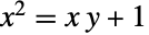
Show[{DiscretizeRegion[ℛ], ContourPlot[x^2 == x y + 1, {x, -2, 3}, {y, -2, 3}],
Plot@@{Last[%[[2]]], {x, First[#], Last[#]}, PlotStyle -> Red}& /@ (List@@%[[1]])}]ℛ = RegionProduct[Circle[], Circle[]];Reduce[Subscript[∃, {a, b}](4 x y a b == 1 && {x, a, y, b}∈ℛ), {x, y}]Subscript[ℛ, 1] = InfiniteLine[{{2, 0}, {0, t}}];
Subscript[ℛ, 2] = Circle[];Reduce[{x, y}∈Subscript[ℛ, 1] && {x, y}∈Subscript[ℛ, 2], {t, x, y}, Reals]
Subscript[ℛ, 1] = Disk[{a, b}];
Subscript[ℛ, 2] = Triangle[{{0, 0}, {0, 5}, {7, 0}}];
Reduce[Subscript[∀, {x, y}, {x, y}∈Subscript[ℛ, 1]]{x, y}∈Subscript[ℛ, 2], {a, b}, Reals]


ℛ = RegionIntersection[Circle[], Line[{{-2, -1}, {1, 2}}]];Reduce[x∈ℛ, x]

ℛ = Sphere[];Reduce[x.{1, 2, 3} == 0 && x∈ℛ, x]オプション (7)
Backsubstitution (1)
Cubics (1)
GeneratedParameters (1)
Reduceは,解を表すために新たなパラメータを導入することがある:
Reduce[Cos[x] == 1 / 2, x]GeneratedParametersを使ってパラメータの生成方法を制御する:
Reduce[Cos[x] == 1 / 2, x, GeneratedParameters -> (Subscript[k, #]&)]Method (1)
次は,"InequalitySolvingOptions"グループと"ReduceOptions"グループのシステムオプションをローカルに設定する:
Reduce[y^5 - 3 y^2 + x^5 + 4 == 0 && y^2 + y - x^5 - 3 x - 11 == 0, {x, y}, Reals, Backsubstitution -> True, Method -> {"AlgebraicNumberOutput" -> False}]デフォルトで,ReduceはここでAlgebraicNumberオブジェクトを使って会を表す:
Reduce[y^5 - 3 y^2 + x^5 + 4 == 0 && y^2 + y - x^5 - 3 x - 11 == 0, {x, y}, Reals, Backsubstitution -> True]Modulus (1)
Quartics (1)
WorkingPrecision (1)
TimeConstrained[Reduce[x^77 + 3 x - 11 == E && y^5 - x^2 y + 21 == π && x^2 y^3 + z^4 == E^π, {x, y, z}, Reals], 60]WorkingPrecision->100を使うと,Reduceは速く解を求められるようになるが,求まった解は正しくないかもしれない:
Timing[Reduce[x^77 + 3 x - 11 == E && y^5 - x^2 y + 21 == π && x^2 y^3 + z^4 == E^π, {x, y, z}, Reals, WorkingPrecision -> 100]]アプリケーション (9)
基本的なアプリケーション (1)


triangle = a > 0 && b > 0 && c > 0 && a + b > c && a + c > b && b + c > a;
acute = a ^ 2 + b ^ 2 > c ^ 2 && a ^ 2 + c ^ 2 > b ^ 2 && b ^ 2 + c ^ 2 > a ^ 2;
s = 1 / 2(a + b + c);
F = Sqrt[s(s - a)(s - b)(s - c)];Reduce[ForAll[{a, b, c}, triangle, a b c(a ^ 2 / b ^ 2 + b ^ 2 / c ^ 2 + c ^ 2 / a ^ 2) ≥ a ^ 3 + b ^ 3 + c ^ 3 + a b(b - a) + a c(a - c) + b c(c - b)]]Reduce[ForAll[{a, b, c}, triangle && acute, 27(b ^ 2 + c ^ 2 - a ^ 2) ^ 2(a ^ 2 + c ^ 2 - b ^ 2) ^ 2(a ^ 2 + b ^ 2 - c ^ 2) ^ 2 ≤ (4F) ^ 6]]多項式の根に関する問題 (1)
f[x_] := x ^ 4 + a x ^ 3 + b x ^ 2 + c x + dReduce[Exists[x, f[x] == 0, ForAll[y, f[y] == 0, x == y]], {a, b, c, d}]Subresultantsを使う:
Reduce[Thread[Drop[Subresultants[f[x], D[f[x], x], x], -1] == 0], {a, b, c, d}, Backsubstitution -> True]パラメータ化問題 (1)
curve = x ^ 2 + y ^ 2 + z ^ 2 == 1 && x ^ 3 + x y ^ 2 == z ^ 2;red = Reduce[curve, {x, y, z}, Reals]bound = N[First[red]]pieces = {x, y, z} //. {ToRules[Rest[red]]}ParametricPlot3D[pieces, {x, First[bound], Last[bound]}]

proj = Reduce[Exists[z, curve], {x, y}, Reals]bounds = N[First[proj]]pieces2d = {x, y} //. {ToRules[Rest[proj]]}ParametricPlot[pieces2d, {x, First[bounds], Last[bounds]}]整数問題 (3)
Reduce[x ^ 2 + y ^ 2 == 5 ^ 2 && y > x > 0, {x, y}, Integers]Table[Reduce[x ^ 2 + y ^ 2 == z ^ 2 && y > x > 0, {x, y}, Integers], {z, 30}]2ドル27セントの郵送料を払うための,10セント,23セント,27セントの切手の組合せ方を求める:
Reduce[a 10 + b 23 + c 37 == 227 && a >= 0 && b >= 0 && c >= 0, {a, b, c}, Integers]IntegerPartitionsを使っても同じタスクを行うことができる:
IntegerPartitions[227, All, {37, 23, 10}]Show[PolyhedronData[#], ImageSize -> Tiny]& /@ PolyhedronData["Platonic"]正  面体の各面は
  本の辺に囲まれているが,どの辺も共有されていて2回ずつ数えられる:
e = (1/2)(n f);正  面体の各面には
  個の頂点があるが,頂点は共有されていて
  回ずつ数えられる:
v = (1/m)(n f);オイラー(Euler)の公式  を使って面の数を求めることができる:
Reduce[f - e + v == 2 && m ≥ 3 && n ≥ 3, f, Reals]この最後の公式がうまく定義されるためには分母が正の整数である必要がある:
Reduce[2 m + 2 n - m n > 0 && m ≥ 3 && n ≥ 3, {m, n}, Integers]{f, e, v} /. f -> -(4 m/-2 m - 2 n + m n) /. FindInstance[2 m + 2 n - m n > 0 && m ≥ 3 && n ≥ 3, {m, n}, Integers, 5]//SortこれをPolyhedronDataの実際の数と比較する:
Table[{PolyhedronData[p, "FaceCount"], PolyhedronData[p, "EdgeCount"], PolyhedronData[p, "VertexCount"]}, {p, PolyhedronData["Platonic"]}]//Sort幾何学問題 (3)
 が真であれば,領域 ℛ は の部分集合である.Disk[{0,0},{2,1}]がRectangle[{-2,-1},{2,1}]の部分集合であることを示す:
ℛ = Disk[{0, 0}, {2, 1}];
𝒮 = Rectangle[{-2, -1}, {2, 1}];Reduce[Subscript[∀, {x, y}]{x, y}∈ℛ{x, y}∈𝒮, Reals]Graphics[{{LightRed, EdgeForm[Gray], 𝒮}, {LightBlue, EdgeForm[Gray], ℛ}}]Cylinder[]⊆Ball[{0,0,0},2]を示す:
ℛ = Cylinder[];
𝒮 = Ball[{0, 0, 0}, 2];Reduce[Subscript[∀, {x, y, z}]{x, y, z}∈ℛ{x, y, z}∈𝒮, Reals]Graphics3D[{{Opacity[0.3], 𝒮}, {LightBlue, EdgeForm[Gray], ℛ}}]有限点集合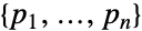 については,点
  についてのボロノイ(Voronoi)セルは
 で定義される.これは,
 のとき,他のすべての点
  より
より  に近いすべての点に相当する.Reduceを使ってボロノイセルの簡単な式を求める:
pts = {{0, 0}, {1, 0}, {1, 1}, {2, 0}};voronoi1 = And@@Table[EuclideanDistance[pts[[1]], {x, y}] <= EuclideanDistance[pts[[j]], {x, y}], {j, 2, 4}]Reduce[voronoi1, {x, y}, Reals]RegionPlot[%, {x, -1, 1}, {y, -1, 1}]vcells = And@@@Table[EuclideanDistance[pts[[i]], {x, y}] <= EuclideanDistance[pts[[j]], {x, y}], {i, 4}, {j, Complement[Range[4], {i}]}];vscells = Reduce[#, {x, y}, Reals]& /@ vcellsRegionPlot[Evaluate@Table[vscells[[i]], {i, 4}], {x, -1, 3}, {y, -1, 3}, PlotLegends -> SwatchLegend[Map[Style[#, Small]&, vscells]], Epilog -> Point[pts]]特性と関係 (10)
syst = x ^ 2 + y ^ 2 + z ^ 2 ≤ 1 && 2x y > z ^ 2;red = Reduce[syst, {x, y, z}, Reals]SeedRandom[0];Table[{syst, red} /. {x -> RandomReal[{-1, 1}], y -> RandomReal[{-1, 1}], z -> RandomReal[{-1, 1}]}, {10}]ToRulesとReplaceRepeatedを使って有限解集合を置換し直すことができる:
Reduce[x ^ 2 + y == 1 && x ^ 2 - y ^ 2 == 2, {x, y}]x ^ 2 + y == 1 && x ^ 2 - y ^ 2 == 2 //. {ToRules[%]}Expandを使って簡単な根基を含む置換の結果を簡約する:
Expand[%]代数的数を含む式の簡約にRootReduceを使う:
Reduce[x ^ 2 + y ^ 2 == 1 && x ^ 3 - 2y ^ 3 == 3, {x, y}]RootReduce[x ^ 2 + y ^ 2 == 1 && x ^ 3 - 2y ^ 3 == 3 //. {ToRules[%]}]FindInstanceを使って解の例を求める:
FindInstance[x ^ 2 + y ^ 2 + z ^ 2 ≤ 1 && 2x y > z ^ 2, {x, y, z}, Reals]FindInstance[x ^ 2 - 3y ^ 2 == 1 && 0 < x < 10 ^ 10, {x, y}, Integers, 3]Solveは複雑な方程式の解を置換規則で表す:
Solve[x ^ 2 + y ^ 2 == 1 && 2x + 3y == 1, {x, y}]Solveはパラメータについての方程式を含む解を除外する:
Reduce[a x ^ 2 + x == 1, x]Solve[a x ^ 2 + x == 1, x]超越方程式については,Solveがすべての解を与えないことがある:
Solve[x + E ^ x == 1 / 2, x]
Reduce[x + E ^ x == 1 / 2, x]逆関数を使うとSolveがある種の解を求めるのが速くなる:
Solve[x ^ n == 1, x]//Timing
完全な解を求めるのには時間がかかり,解自体も長くなることがある:
(red = Reduce[x ^ n == 1, x])//LeafCount//Timing
Reduce[red /. x -> 2, n]Simplify[x ^ n /. {x -> 2, n -> 2I Pi C[1] / Log[2]}, Element[C[1], Integers]]SolveAlwaysは複雑な式が常に真であるパラメータの値を返す:
SolveAlways[(a - 2b + 1)x ^ 2 + (a - b ^ 2 - c)x == a ^ 2 - b + 3c - 1, x]次は,同じ問題をReduceを使って解く:
Reduce[ForAll[x, (a - 2b + 1)x ^ 2 + (a - b ^ 2 - c)x == a ^ 2 - b + 3c - 1], {a, b, c}]Resolveは限定子を除去するが,必ずしも結果の限定子を含まない式を解く訳ではない:
Resolve[Exists[x, x ^ 2 + y ^ 2 + z ^ 2 == 1 && x y > z ^ 3], Reals]Resolve[ForAll[{x, y}, a x ^ 2 + b x + c == 0 && a y ^ 2 + b y + c == 0, x == y]]Eliminateは複雑な方程式の系から変数を除去する:
Eliminate[x ^ 2 + y ^ 2 + z ^ 2 == 1 && x y == z ^ 3, x]以下では同じ問題をResolveを使って解いている:
Resolve[Exists[x, x ^ 2 + y ^ 2 + z ^ 2 == 1 && x y == z ^ 3]]Reduceは結果の方程式も解く:
Reduce[Exists[x, x ^ 2 + y ^ 2 + z ^ 2 == 1 && x y == z ^ 3], {y, z}]考えられる問題 (5)
 は不等式に含まれているので,実数だと仮定される.
 は複素数でもよい:
Reduce[x ^ 2 < 1 && y - Sqrt[x] == 0, {x, y}]領域Realsが指定されると, ,
, それにSqrt[x]は実数でなければならなくなる:
Reduce[x ^ 2 < 1 && y - Sqrt[x] == 0, {x, y}, Reals]
Reduce[x ^ 2 < 1 && y - Sqrt[x] == 0, {x, y}, Complexes]変数の次数が問題の可解性に影響することがある.以下は, に関して
に関して  について簡単に解くことがでる:
Reduce[y == x - Sin[x], {x, y}]

Reduce[y == x - Sin[x], {y, x}]
ReduceはWolfram言語関数の分枝切断線に依存する方程式を解かない:
Reduce[Sqrt[x + 2y] - x ^ 2 + y - 1 == 0, {x, y}]
Block[{x = u + I v}, RegionPlot[Abs[-1 + Sqrt[3 + x + 2 x^2] - Sqrt[4 + x + 2 x^2 - 2 Sqrt[3 + x + 2 x^2]]] > 0.001, {u, -10, 10}, {v, -10, 10}]]Reduceは,部分式の実数領域の外に属する実数解を求めない:
Reduce[z > 0 && Im[HankelH1[0, z]] == 0, z, Reals]Reduceは数学関数の実数領域を決定するためにFunctionDomain を用いる:
FunctionDomain[HankelH1[0, z], z]FunctionDomainは,低次元集合を除いて正確な実数領域の情報を有する:
Plot[Im[HankelH1[0, z]], {z, -3, 3}]HankelH1[0,z]が実数値となる孤立点が存在する:
N[HankelH1[0, BesselYZero[0, 1]], 20]Reduce[(x ^ 2 - 2Sqrt[2]x + 2) / (x - Sqrt[2]) == 0, x]Limit[(x ^ 2 - 2Sqrt[2]x + 2) / (x - Sqrt[2]), x -> Sqrt[2]]しかし,解には自動簡約で削除される可除特異点が含まれることがある:
Reduce[x ^ 2 / x == 0, x]
x ^ 2 / x == 0以下では  における可除特異点が方程式の前処理に使われたTogetherによって削除されている:
Reduce[(x ^ 2 - 2x + 1) / (x - 1) == 0, x]Together[(x ^ 2 - 2x + 1) / (x - 1) == 0]
テキスト
Wolfram Research (1988), Reduce, Wolfram言語関数, https://reference.wolfram.com/language/ref/Reduce.html (2024年に更新).
CMS
Wolfram Language. 1988. "Reduce." Wolfram Language & System Documentation Center. Wolfram Research. Last Modified 2024. https://reference.wolfram.com/language/ref/Reduce.html.
APA
Wolfram Language. (1988). Reduce. Wolfram Language & System Documentation Center. Retrieved from https://reference.wolfram.com/language/ref/Reduce.html