

Projection
Projection[u,v]
finds the projection of the vector u onto the vector v.
Projection[u,{v1,v2,…}]
finds the projection of u onto the subspace spanned by the vectors vi.
Projection[u,v,f]
finds projections with respect to the inner product function f.
Details

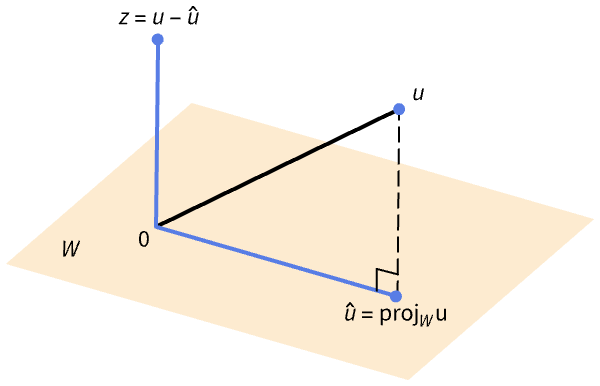
- Projection computes the orthogonal projection of a vector u onto a subspace
 in an inner product space.
 - Orthogonal projections play an important role in linear regression and, more generally, in applications involving the method of least squares.
- For ordinary real vectors u and v, the projection is taken to be
 .
. - For ordinary complex vectors u and v, the projection is taken to be
 , where
  is Conjugate[v]. »
 - In Projection[u,v,f], u and v can be any expressions or lists of expressions for which the inner product function f applied to pairs yields real results. »
- Projection[u,v,Dot] effectively assumes that all elements of u and v are real. »
- Projection[u,{v1,v2,…}] projects u onto the subspace spanned by the vi. This usage does not accept a third argument.
- Projection[u,{v1,v2,…,vm}] is defined by
![sum_(i=1)^mTemplateBox[{{e, _, i}}, Conjugate].u e_i](Files/Projection.en/6.png "sum_(i=1)^mTemplateBox[{{e, _, i}}, Conjugate].u e_i") , where {e1,e2,…,em}=Orthogonalize[{v1,v2,…,vm}]. »
, where {e1,e2,…,em}=Orthogonalize[{v1,v2,…,vm}]. »
Examples
open all close allBasic Examples (3)
Scope (14)
Basic Uses (6)
Projections onto Subspaces (5)
Projection of the vector ![]() onto the subspace spanned by
onto the subspace spanned by ![]() and
and ![]() :
:
Projection of a complex vector onto a subspace:
Project a vector onto a three-dimensional subspace at machine precision:
Projection of large numerical vectors onto a subspace is computed efficiently:
Project a symbolic vector onto a symbolic subspace, assuming real variables:
General Inner Products (3)
Give an inner product of Dot to assume all expressions are real-valued:
Project vectors that are not lists using an explicit inner product:
Applications (18)
Geometry (4)
Project the vector ![]() on the line spanned by the vector
on the line spanned by the vector ![]() :
:
Visualize ![]() and its projection onto the line spanned by
and its projection onto the line spanned by ![]() :
:
Project the vector ![]() on the plane spanned by the vectors
on the plane spanned by the vectors ![]() and
and ![]() :
:
The projection on the plane is given by:
Notice that this is not simply the sum of the projections onto the ![]() :
:
Find the component perpendicular to the plane:
Confirm the result by projecting ![]() onto the normal to the plane:
onto the normal to the plane:
Visualize the plane, the vector and its parallel and perpendicular components:
Use Projection to reflect the vector ![]() with respect to the line normal to the vector
with respect to the line normal to the vector ![]() :
:
Since ![]() is perpendicular to the line, subtracting twice
is perpendicular to the line, subtracting twice ![]() will reflect
will reflect ![]() across the line:
across the line:
Compare with the result of ReflectionTransform:
Visualize ![]() and its reflection as a twice-repeated translation by
and its reflection as a twice-repeated translation by ![]() :
:
The Frenet–Serret system encodes every space curve's properties in a vector basis and scalar functions. Consider the following curve (a helix):
Construct an orthonormal basis from the first three derivatives by subtracting parallel projections:
Ensure that the basis is right-handed:
Compute the curvature, ![]() , and torsion,
, and torsion, ![]() , which quantify how the curve bends:
, which quantify how the curve bends:
Verify the answers using FrenetSerretSystem:
Visualize the curve and the associated moving basis, also called a frame:
Bases and Matrix Decompositions (3)
Apply the Gram–Schmidt process to construct an orthonormal basis from the following vectors:
The first vector in the orthonormal basis, ![]() , is merely the normalized multiple
, is merely the normalized multiple ![]() :
:
For subsequent vectors, components parallel to earlier basis vectors are subtracted prior to normalization:
Confirm the answers using Orthogonalize:
Find an orthonormal basis for the column space of the following matrix ![]() , and then use that basis to find a QR factorization of
, and then use that basis to find a QR factorization of ![]() :
:
Define ![]() as the
as the ![]() element of the corresponding Gram–Schmidt basis:
element of the corresponding Gram–Schmidt basis:
Define ![]() as the matrix whose columns are
as the matrix whose columns are ![]() :
:
Compare with the result given by QRDecomposition; the ![]() matrices are the same:
matrices are the same:
The ![]() matrices differ by a transposition because QRDecomposition gives the row-orthonormal result:
matrices differ by a transposition because QRDecomposition gives the row-orthonormal result:
For a Hermitian matrix (more generally, any normal matrix), the eigenvectors are orthogonal, and it is conventional to define the projection matrices ![]() , where
, where ![]() is a normalized eigenvector. Show that the action of the projection matrices on a general vector is the same as projecting the vector onto the eigenspace for the following matrix
is a normalized eigenvector. Show that the action of the projection matrices on a general vector is the same as projecting the vector onto the eigenspace for the following matrix ![]() :
:
Find the eigenvalues and eigenvectors:
Compute the normalized eigenvectors:
Compute the projection matrices:
Confirm that multiplying a general vector by ![]() equals the projection of the vector onto
equals the projection of the vector onto ![]() :
:
Since the ![]() form an orthonormal basis, the sum of the
form an orthonormal basis, the sum of the ![]() must be the identity matrix:
must be the identity matrix:
Least Squares and Curve Fitting (3)
If the linear system ![]() has no solution, the best approximate solution is the least-squares solution. That is the solution to
has no solution, the best approximate solution is the least-squares solution. That is the solution to ![]() , where
, where ![]() is the orthogonal projection of
is the orthogonal projection of ![]() onto the column space of
onto the column space of ![]() . Consider the following
. Consider the following ![]() and
and ![]() :
:
The linear system is inconsistent:
Find orthogonal vectors that span ![]() . First, let
. First, let ![]() be the first column of
be the first column of ![]() :
:
Let ![]() be a vector in the column space that is perpendicular to
be a vector in the column space that is perpendicular to ![]() :
:
Compute the orthogonal projection ![]() of
of ![]() onto the spaced spanned by the
onto the spaced spanned by the ![]() :
:
Note that this could have been computed directly by projecting onto ![]() computed with RangeSpace:
computed with RangeSpace:
Visualize ![]() , its projections
, its projections ![]() onto the
onto the ![]() and
and ![]() :
:
Confirm the result using LeastSquares:
Projection can be used to find a best-fit curve to data. Consider the following data:
Extract the ![]() and
and ![]() coordinates from the data:
coordinates from the data:
Let ![]() have the columns
have the columns ![]() and
and ![]() , so that minimizing
, so that minimizing ![]() will be fitting to a line
will be fitting to a line ![]() :
:
The following two orthogonal vectors clearly span the same spaces as the column of ![]() :
:
Get the coefficients ![]() and
and ![]() for a linear least‐squares fit:
for a linear least‐squares fit:
Verify the coefficients using Fit:
Plot the best-fit curve along with the data:
Find the best-fit parabola to the following data:
Extract the ![]() and
and ![]() coordinates from the data:
coordinates from the data:
Let ![]() have the columns
have the columns ![]() ,
, ![]() and
and ![]() , so that minimizing
, so that minimizing ![]() will be fitting to
will be fitting to ![]() :
:
Construct orthonormal vectors ![]() that have the same column space as
that have the same column space as ![]() :
:
Get the coefficients ![]() ,
, ![]() and
and ![]() for a least‐squares fit:
for a least‐squares fit:
Verify the coefficients using Fit:
General Inner Products and Function Spaces (5)
A positive-definite, real symmetric matrix or metric ![]() defines an inner product by
defines an inner product by ![]() :
:
Being positive-definite means that the associated quadratic form ![]() is positive for
is positive for ![]() :
:
Note that Dot itself is the inner product associated with the identity matrix:
Apply the Gram–Schmidt process to the standard basis to obtain an orthonormal basis:
Confirm that this basis is orthonormal with respect to the inner product ![]() :
:
Fourier series are projections onto a particular basis in the inner product spaces ![]() . Define the standard inner product on square-integrable functions:
. Define the standard inner product on square-integrable functions:
Let ![]() denote
denote ![]() for different integer values of
for different integer values of ![]() :
:
The ![]() are orthogonal to each other, though not orthonormal:
are orthogonal to each other, though not orthonormal:
The Fourier series of a function ![]() is the projection of
is the projection of ![]() onto the space spanned by the
onto the space spanned by the ![]() :
:
Confirm the result using FourierSeries:
Moreover, ![]() equals the Fourier coefficient corresponding to FourierParameters{-1,1}:
equals the Fourier coefficient corresponding to FourierParameters{-1,1}:
Confirm using FourierCoefficient:
Unnormalized Gram–Schmidt algorithm:
Do Gram–Schmidt on a random set of 3 vectors:
Verify orthogonality; as the vectors are not normalized, the result is a general diagonal matrix:
Use a positive and real symmetric matrix to define a complex inner product:
Do Gram–Schmidt on a random set of three complex vectors:
LegendreP defines a family of orthogonal polynomials with respect to the inner product ![]() . Apply the unnormalized Gram–Schmidt process to the monomials
. Apply the unnormalized Gram–Schmidt process to the monomials ![]() for
for ![]() from zero through four to compute scalar multiples of the first five Legendre polynomials:
from zero through four to compute scalar multiples of the first five Legendre polynomials:
Compare ![]() to the conventional Legendre polynomials:
to the conventional Legendre polynomials:
For each ![]() ,
, ![]() and
and ![]() differ by a constant multiple, which can be shown to equal
differ by a constant multiple, which can be shown to equal ![]() :
:
Compare with an explicit expression for the orthonormalized polynomials:
HermiteH defines a family of orthogonal polynomials with respect to the inner product ![]() . Apply the unnormalized Gram–Schmidt process to the monomials
. Apply the unnormalized Gram–Schmidt process to the monomials ![]() for
for ![]() from zero through four to compute scalar multiples of the first four Hermite polynomials:
from zero through four to compute scalar multiples of the first four Hermite polynomials:
Compared to the conventional Hermite polynomials, ![]() is smaller by a factor of
is smaller by a factor of ![]() :
:
The orthonormal polynomials differ by a multiple of ![]() in the denominator:
in the denominator:
Compare with an explicit expression for the orthonormalized polynomials:
Quantum Mechanics (3)
In quantum mechanics, states are represented by complex unit vectors and physical quantities by Hermitian linear operators. The eigenvalues represent possible observations and the squared norm of projections onto the eigenvectors the probabilities of those observations. For the spin operator ![]() and state
and state ![]() given, find the possible observations and their probabilities:
given, find the possible observations and their probabilities:
Computing the eigensystem, the possible observations are ![]() :
:
The relative probabilities are ![]() for
for ![]() and
and ![]() for
for ![]() :
:
In quantum mechanics, the energy operator is called the Hamiltonian ![]() , and a state with energy
, and a state with energy ![]() evolves according to the Schrödinger equation
evolves according to the Schrödinger equation ![]() . Given the Hamiltonian for a spin-1 particle in a constant magnetic field in the
. Given the Hamiltonian for a spin-1 particle in a constant magnetic field in the ![]() direction, find the state at time
direction, find the state at time ![]() of a particle that is initially in the state
of a particle that is initially in the state ![]() representing
representing ![]() :
:
Computing the eigensystem, the energy levels are ![]() and
and ![]() :
:
The state at time ![]() is the sum of each eigenstate evolving according to the Schrödinger equation:
is the sum of each eigenstate evolving according to the Schrödinger equation:
For the Hamiltonian ![]() , the
, the ![]() eigenvector is a function that is a constant multiple of
eigenvector is a function that is a constant multiple of ![]() , and the inner product on vectors is
, and the inner product on vectors is ![]() . For a particle in the state
. For a particle in the state ![]() , find the probability that it is in one of the first four eigenstates. First, define an inner product:
, find the probability that it is in one of the first four eigenstates. First, define an inner product:
Confirm that ![]() is a unit vector in this inner product:
is a unit vector in this inner product:
Project onto the first four states; for ![]() and
and ![]() , the projection and hence probability is zero:
, the projection and hence probability is zero:
The probability is given by the squared norm of the projection. For ![]() , it is just under 90%:
, it is just under 90%:
Properties & Relations (14)
The projection of u onto v is in the direction of v:
The projection of v onto itself is v:
Projecting onto a vector and projecting onto the subspace defined by a vector are the same operation:
If w is any linear combination of vectors vi, the projection of w onto the subspace spanned by the vi is w:
For ordinary vectors ![]() and
and ![]() , the projection is taken to be
, the projection is taken to be ![]() :
:
If vi are mutually orthogonal, Projection[u,{v1,v2,…,vn}] can be computed as ![]() :
:
This formula is often written using TensorProduct as ![]() :
:
Note that this is simply the sum of the projections onto the individual vectors:
For vectors u and v, u-Projection[u,v] is orthogonal to v:
The vector u-Projection[u,{v1,v2,…}] is orthogonal to any linear combination of the vi:
If ![]() and
and ![]() have real entries,
have real entries, ![]() , where
, where ![]() is the angle between
is the angle between ![]() and
and ![]() :
:
Orthogonalize can be implemented by repeated application of Projection and Normalize:
For ordinary vectors ![]() and
and ![]() , the projection can be computed as
, the projection can be computed as ![]() :
:
The projection of u onto v is equivalent to multiplication by an outer product matrix:
Note that m is a square matrix:
In the complex case, two instances of v are replaced by Conjugate[v]:
The projection of u onto {v1,v2,…}Transpose[m] equals m.PseudoInverse[m].u:
Text
Wolfram Research (2007), Projection, Wolfram Language function, https://reference.wolfram.com/language/ref/Projection.html (updated 2025).
CMS
Wolfram Language. 2007. "Projection." Wolfram Language & System Documentation Center. Wolfram Research. Last Modified 2025. https://reference.wolfram.com/language/ref/Projection.html.
APA
Wolfram Language. (2007). Projection. Wolfram Language & System Documentation Center. Retrieved from https://reference.wolfram.com/language/ref/Projection.html