Wolfram言語＆システムドキュメントセンター

CentralMoment

CentralMoment[data,r]

data の r 次中心モーメントを与える．

CentralMoment[data,{r₁,…,r_m}]

data の次数が{r₁,…,r_m}の多変量中心モーメントを与える．

CentralMoment[dist,…]

分布 dist の中心モーメントを与える．

CentralMoment[r]

r 次の形式的な中心モーメントを表す．

CentralMoment

CentralMoment[data,r]

data の r 次中心モーメントを与える．

CentralMoment[data,{r₁,…,r_m}]

data の次数が{r₁,…,r_m}の多変量中心モーメントを与える．

CentralMoment[dist,…]

分布 dist の中心モーメントを与える．

CentralMoment[r]

r 次の形式的な中心モーメントを表す．

詳細

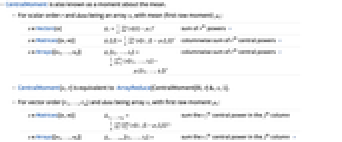
CentralMomentは平均まわりのモーメントとしても知られている．
次数 r のスカラー，data は配列，平均（最初の生のモーメント）では以下のようになる．
r 次ベキの和 »

列ごとの r 次中心ベキの和 »

$x in TemplateBox[{Arrays, paclet:ref/Arrays}, RefLink, BaseStyle -> {3ColumnTableMod}][{n_(1),...,n_(k)}]$ 列ごとの r 次中心ベキの和 »
CentralMoment[x,r]はArrayReduce[CentralMoment[#,r]&,x,1]に等しい．
次数{r₁,…,r_m}のベクトル， data は配列，最初の生のモーメントでは以下のようになる．
第 j 列の r_j次中心ベキの和

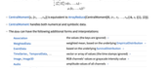
$x in TemplateBox[{Arrays, paclet:ref/Arrays}, RefLink, BaseStyle -> {3ColumnTableMod}][{n_(1),...,n_(k)}]$ 第 j 列の r_j次中心ベキの和　 »
CentralMoment[x,{r₁,…,r_m}]はArrayReduce[CentralMoment[#, ${r_1,r_2,...,r_m}$ ]&,x,{{1},{2}}]に等しい．
CentralMomentは数値データと記号データの両方を扱うことができる．
data は，次の追加的な形式と解釈を持つことができる．

	Association	値（キーは無視される） »
	WeightedData	もとになっているEmpiricalDistributionに基づいた加重平均 »
	EventData	もとになっているSurvivalDistributionに基づく »
	TimeSeries, TemporalData, …	値のベクトルまたは配列（タイムスタンプは無視される） »
	Image,Image3D	RGBチャンネルの値またはグレースケールの強度値 »
	Audio	すべてのチャンネルの振幅値 »
	DateObject, TimeObject	日付のリストまたは時間のリスト »

分布 dist について，r 次中心モーメントはExpectation[(x-Mean[dist])^r,xdist]で与えられる． »
多変量分布 dist について，{r₁,…,r_m}次中心モーメントはExpectation[(x₁-μ₁)^r₁⋯(x₂-μ_m)^r_m,{x₁,…,x_m}dist]および{μ₁,…,μ_m}=Mean[dist]で与えられる． »
ランダム過程 proc については，中心モーメント関数は時点 t におけるスライス分布SliceDistribution[proc,t]について [t]=CentralMoment[SliceDistribution[proc,t],r]として計算することができる． »
CentralMoment[r]は，MomentConvert，MomentEvaluate等の関数とともに使うことができる． »

例題

すべて開くすべて閉じる

例 (3)

データから中心モーメントを計算する：

Wolfram Language code: data = RandomVariate[LogNormalDistribution[1, 1], 10 ^ 5];

Wolfram Language code: CentralMoment[data, 3]

記号データを使う：

Wolfram Language code: CentralMoment[{Subscript[x, 1], Subscript[x, 2], Subscript[x, 3]}, 2]

日付のリストの中心モーメント：

Wolfram Language code: CentralMoment[{Yesterday, Today, Tomorrow}, 4]

一変量分布の二次中心モーメントを計算する：

Wolfram Language code: CentralMoment[GammaDistribution[α, β], 2]

多変量分布の中心モーメント：

Wolfram Language code: CentralMoment[DirichletDistribution[{Subscript[α, 1], Subscript[α, 2], Subscript[α, 3]}], {1, 1}]

スコープ (26)

基本的な用法 (6)

厳密な入力は厳密な出力を与える：

Wolfram Language code: CentralMoment[{1, 2, 3, 4}, 4]

Wolfram Language code: CentralMoment[{π, E, 2}, 2]//Together

近似入力は近似出力を与える：

Wolfram Language code: CentralMoment[{1., 2., 3., 4.}, 2]

Wolfram Language code: CentralMoment[N[{1, 2, 3, 4}, 30], 2]

WeightedDataの中心モーメントを求める：

Wolfram Language code: CentralMoment[WeightedData[{1, 2, 3}, {Subscript[w, 1], Subscript[w, 2], Subscript[w, 3]}], 2]

Wolfram Language code:

data = {8, 3, 5, 4, 9, 0, 4, 2, 2, 3};
weights = {0.15, 0.09, 0.12, 0.10, 0.16, 0., 0.11, 0.08, 0.08, 0.09};

Wolfram Language code: CentralMoment[WeightedData[data, weights], 2]

EventDataの中心モーメントを求める：

Wolfram Language code:

e = {1.0, 2.1, 3.2, 4.5, 5.7};
ci = {0, 0, 0, 1, 0};

Wolfram Language code: CentralMoment[EventData[e, ci], 2]

TimeSeriesの中心モーメントを求める：

Wolfram Language code:

CentralMoment[TemporalData[TimeSeries, {{{2.3, 1.2, 6.7, 5.8, 7.1, 4.6}}, {{0, 5, 1}}, 1, {"Discrete", 1}, 
  {"Discrete", 1}, 1, {}}, False, 10.], 2]

中心モーメントは値のみに依存する：

Wolfram Language code:

CentralMoment[TemporalData[TimeSeries, {{{2.3, 1.2, 6.7, 5.8, 7.1, 4.6}}, {{0, 5, 1}}, 1, {"Discrete", 1}, 
  {"Discrete", 1}, 1, {}}, False, 10.]["Values"], 2]

数量を含むデータについての中心モーメントを求める：

Wolfram Language code: data = Quantity[RandomReal[1, 6], "Meters"]

Wolfram Language code: CentralMoment[data, 2]

配列データ (5)

行列についてのCentralMomentは列ごとのモーメントを返す：

Wolfram Language code:

CentralMoment[(⁠|       |       |
| ----- | ----- |
| a1, 1 | a1, 2 |
| a2, 1 | a2, 2 |⁠), 4]//Simplify

配列についてのCentralMomentは第1レベルの列ごとのモーメントを返す：

Wolfram Language code: CentralMoment[Array[Subscript[a, ##]&, {2, 2, 2}], 2]//Simplify//MatrixForm

配列についての多変量CentralMoment：

Wolfram Language code: CentralMoment[Array[Subscript[a, ##]&, {2, 2, 2}], {2, 2}]//Simplify

大きい配列に使うことができる：

Wolfram Language code: CentralMoment[RandomReal[1, 10 ^ 7], 2]

Wolfram Language code: CentralMoment[RandomReal[1, {10 ^ 6, 5}], 2]

入力がAssociationのとき，CentralMomentはその値に作用する：

Wolfram Language code:

mat = RandomReal[1, {3, 2}];
assoc = AssociationThread[Range[3], mat]

Wolfram Language code: CentralMoment[assoc, 3]

SparseArrayデータは密な配列のように使うことができる：

Wolfram Language code: CentralMoment[SparseArray[{{1} -> 1, {100} -> 1}], 4]

Wolfram Language code: CentralMoment[SparseArray[{{1, 1} -> 1, {2, 2} -> 2, {3, 3} -> 3, {1, 3} -> 4}], 2]

QuantityArrayの中心モーメントを求める：

Wolfram Language code: data = QuantityArray[RandomReal[1, 6], "Pounds"]

Wolfram Language code: CentralMoment[data, 5]

画像データと音声データ (2)

RGB画像のチャンネルごとの中心モーメント：

Wolfram Language code: CentralMoment[[image], 5]

Wolfram Language code: RGBColor[%]

グレースケール画像の中心モーメント強度値：

Wolfram Language code: CentralMoment[[image], 4]

CentralMomentは，音声オブジェクトについてはチャンネルごとに作用する：

Wolfram Language code: a = ExampleData[{"Audio", "Bee"}]

Wolfram Language code: AudioMeasurements[a, "Channels"]

Wolfram Language code: CentralMoment[a, 3]

日付と時間 (4)

日付の中心モーメントを計算する：

Wolfram Language code: dates = WolframLanguageData[All, "DateIntroduced"];

Wolfram Language code: DateHistogram[dates]

Wolfram Language code: CentralMoment[dates, 4]

Wolfram Language code: UnitConvert[%, "Decades" ^ 4]

日付の重み付き中心モーメントを計算する：

Wolfram Language code: dates = RandomDate[4]

Wolfram Language code: weights = {1, 1, 1, 3};

Wolfram Language code: CentralMoment[WeightedData[dates, weights], 3]

Wolfram Language code: UnitConvert[%, "Years" ^ 3]

異なる暦で与えられた日付の中心モーメントを計算する：

Wolfram Language code:

dates = {DateObject[{2024, 2, 29}, CalendarType -> "Julian"], DateObject[{1524, 1, 1}, CalendarType -> "Islamic"], DateObject[{6024, 1, 15}, CalendarType -> "Jewish"]}

Wolfram Language code: CentralMoment[dates, 2]

Wolfram Language code: UnitConvert[%, "Years" ^ 2]

分散と比較する：

Wolfram Language code: Variance[dates]

Wolfram Language code: UnitConvert[%, "Years" ^ 2]

時間の中心モーメントを計算する：

Wolfram Language code: RandomTime[3]

Wolfram Language code: CentralMoment[%, 4]

異なる時刻帯指定の時刻のリスト：

Wolfram Language code: {TimeObject[{12}, TimeZone -> 0], TimeObject[{12}, TimeZone -> 2], TimeObject[{12}, TimeZone -> "Asia/Tokyo"]}

Wolfram Language code: CentralMoment[%, 3]

分布のモーメントと過程のモーメント (5)

一変量分布のスカラー中心モーメント：

Wolfram Language code: CentralMoment[BinomialDistribution[n, p], 2]//Together

Wolfram Language code: CentralMoment[NormalDistribution[μ, σ], 2]

多変量分布のスカラー中心モーメント：

Wolfram Language code: CentralMoment[BinormalDistribution[{Subscript[μ, 1], Subscript[μ, 2]}, {Subscript[σ, 1], Subscript[σ, 2]}, ρ], 2]

Wolfram Language code: CentralMoment[DirichletDistribution[{a, b, c}], 3]

多変量分布の結合中心モーメント：

Wolfram Language code: CentralMoment[MultinomialDistribution[n, {Subscript[p, 1], Subscript[p, 2], Subscript[p, 3]}], {1, 1, 1}]

Wolfram Language code:

CentralMoment[BinormalDistribution[{Subscript[μ, 1], Subscript[μ, 2]}, {Subscript[σ, 1], Subscript[σ, 2]}, ρ], {2, 2}]

記号次数 r についての中心モーメントを計算する：

Wolfram Language code: CentralMoment[BetaDistribution[a, b], r]

中心モーメントは特定の次数についてしか評価できないことがある：

Wolfram Language code: CentralMoment[ExtremeValueDistribution[a, b], r]

Wolfram Language code: % /. r -> 3

中心モーメントは数値的にしか評価できないことがある：

Wolfram Language code: CentralMoment[VonMisesDistribution[Pi / 2, 2], 4]

Wolfram Language code: N[%]

派生分布についての中心モーメント：

Wolfram Language code: CentralMoment[TransformedDistribution[x^2, xNormalDistribution[μ, σ]], 2]

Wolfram Language code: CentralMoment[ProbabilityDistribution[(Sqrt[2] / π)(1 / (1 + (x - 2)^4)), {x, -∞, ∞}], 2]

データ分布について：

Wolfram Language code: data = RandomVariate[NormalDistribution[], 10 ^ 3];

Wolfram Language code: CentralMoment[HistogramDistribution[data], 4]

ランダム過程についての中心モーメント関数：

Wolfram Language code: CentralMoment[BrownianBridgeProcess[μ, σ][t], 4]

Wolfram Language code: Plot[Evaluate[% /. {μ -> 3, σ -> 1}], {t, 0, 1}, PlotRange -> All]

ある時点 t=0.5におけるTemporalDataの中心モーメントを求める：

Wolfram Language code: td = RandomFunction[WienerProcess[1, 1], {0, 10, 0.05}, 100]

Wolfram Language code: CentralMoment[td[0.5], 2]

対応する中心モーメント関数をすべてのシミュレーションとともに求める：

Wolfram Language code:

Show[ListLinePlot[td, PlotStyle -> Directive[Opacity[0.2], Thin]], Plot[CentralMoment[td[t], 2], {t, 0, 10}, PlotStyle -> Thick]]

形式的なモーメント (4)

形式的なモーメントのTraditionalFormによる表示：

Wolfram Language code: CentralMoment[r]//TraditionalForm

Wolfram Language code: CentralMoment[{p, q, r}]//TraditionalForm

形式的なモーメントの組合せをCentralMomentを含む式に変換する：

Wolfram Language code: MomentConvert[Moment[2], CentralMoment]//TraditionalForm

Wolfram Language code: MomentConvert[Moment[2]Cumulant[2], CentralMoment]//TraditionalForm

形式的なモーメントを含む式を分布について評価する：

Wolfram Language code: MomentEvaluate[CentralMoment[2] + CentralMoment[4], PoissonDistribution[λ]]

データについて評価する：

Wolfram Language code: data = RandomVariate[PoissonDistribution[1], 10^4];

Wolfram Language code: MomentEvaluate[CentralMoment[2] + Moment[4], data]

CentralMomentを含む式のサンプル推定量を求める：

Wolfram Language code: (estimator = MomentConvert[CentralMoment[2], "UnbiasedSampleEstimator"])//TraditionalForm

結果の推定量をデータについて評価する：

Wolfram Language code: data = RandomVariate[PoissonDistribution[1], 10^4];

Wolfram Language code: MomentEvaluate[estimator, data]

アプリケーション (11)

一次中心モーメントは常に0である：

Wolfram Language code: data = RandomReal[{-7, 3}, 100];

Wolfram Language code: CentralMoment[data, 1]

二次中心モーメントは分散度である：

Wolfram Language code: 𝒟 = NormalDistribution[0, σ];

Wolfram Language code: CentralMoment[𝒟, 2]

Wolfram Language code:

Table[Plot[PDF[𝒟, x], {x, -4, 4}, PlotRange -> {0, 0.4}, Filling -> Axis, Ticks -> {Automatic, None}], {σ, {1, 1.5, 2}}]

三次中心モーメントは歪度の尺度である：

Wolfram Language code: dists = {NormalDistribution[0, 2.5], ChiSquareDistribution[5], GumbelDistribution[3, 2]};

Wolfram Language code: Table[CentralMoment[dists[[i]], 3], {i, 3}]//N

Wolfram Language code: Table[Plot[PDF[dists[[i]], x], {x, -7, 15}, PlotRange -> {0, 0.2}, Filling -> Axis, Ticks -> {Automatic, None}], {i, 3}]

モーメント法を使って分布母数を推定する：

Wolfram Language code: data = RandomVariate[GammaDistribution[3, 6], 10 ^ 4];

Wolfram Language code: meq = Table[CentralMoment[data, k] == CentralMoment[GammaDistribution[α, β], k], {k, 2, 3}]

Wolfram Language code: NSolve[meq, {α, β}]

データと推定されたパラメトリック分布を比較する：

Wolfram Language code:

Show[Histogram[data, Automatic, "ProbabilityDensity"], Plot[Evaluate[PDF[GammaDistribution[α, β], x] /. %], {x, 0, 100}, PlotStyle -> Thick]]

モーメント法を使ってGammaDistributionの正規近似を求める：

Wolfram Language code: gdist = GammaDistribution[α, β];

Wolfram Language code:

meq = {Moment[gdist, 1] == Moment[NormalDistribution[μ, σ], 1], CentralMoment[gdist, 2] == CentralMoment[NormalDistribution[μ, σ], 2]}

とがとにいかに依存しているかを示す：

Wolfram Language code: Solve[(And@@meq)∧σ > 0, {μ, σ}, Reals]

Wolfram Language code: {ndist} = Refine[NormalDistribution[μ, σ] /. %, β > 0∧α > 0]

もとの分布と近似された分布を比較する：

Wolfram Language code: Plot[{PDF[gdist, x], PDF[ndist, x]} /. {α -> 13, β -> 3}, {x, 0, 80}, Evaluated -> True]

二次中心モーメントのサンプル推定器を構築する：

Wolfram Language code: estim = MomentConvert[CentralMoment[2], "SampleEstimator"]

サンプルサイズがであると仮定してサンプル分布の期待値を求める：

Wolfram Language code: MomentConvert[estim, {CentralMoment, n}]

推定器のサンプル分布分散を求める：

Wolfram Language code: MomentConvert[(estim - %) ^ 2, {CentralMoment, n}]

一様分布に従うサンプルの推定器の分散：

Wolfram Language code: MomentEvaluate[%, UniformDistribution[{0, 1}]]

大数の法則にはサンプルサイズが増大するにつれてサンプルモーメントが母集団のモーメントに近付くとある．Histogramを使ってさまざまなサンプルサイズについて一様分布に従う確率変量のサンプルの二次中心モーメントの確率分布を示す：

Wolfram Language code:

Histogram[Table[CentralMoment[RandomReal[1, {n, 2 * 10 ^ 3}], 2], {n, {10, 10^2, 10^3}}], 30, "ProbabilityDensity", ChartLegends -> {10, 10^2, 10^3}]

三次および四次中心モーメントを訂正するほぼ正規分布に従うデータのエッジワース(Edgeworth)展開：

Wolfram Language code:

pdf = (Exp[-(x^2/2)]/Sqrt[2 π]) (1 + ((-6 Sqrt[2] x + 2 Sqrt[2] x^3) CentralMoment[3]/12 Sqrt[2]) + (1/576) (-120 + 360 x^2 - 120 x^4 + 8 x^6) CentralMoment[3]^2 + (1/96) (12 - 24 x^2 + 4 x^4) (-3 + CentralMoment[4]));

Wolfram Language code: data = Standardize[Total[RandomReal[1, {3, 10 ^ 5}]]];

Wolfram Language code: dist = ProbabilityDistribution[MomentEvaluate[pdf, data], {x, -∞, ∞}]

Wolfram Language code: {NExpectation[x ^ 3, xdist], NExpectation[x ^ 4, xdist]}

Wolfram Language code: {CentralMoment[data, 3], CentralMoment[data, 4]}

Wolfram Language code:

Show[Histogram[data, Automatic, "ProbabilityDensity"], Plot[{PDF[dist, z], PDF[NormalDistribution[], z]}, {z, -3, 3}, PlotStyle -> {Directive[Thick], Directive[Dashed, Red]}]]

Jarque–Bera統計サンプルを計算する関数 [リンク]：

Wolfram Language code:

JarqueBera[list_] := With[{cm2 = CentralMoment[list, 2]}, (Length[list]/6)((CentralMoment[list, 3]^2/cm2^3) + (1/4)((CentralMoment[list, 4]/cm2^2) - 3)^2)]

正規分布に従う確率変量のサンプルについての累積統計：

Wolfram Language code: data = Table[JarqueBera[RandomVariate[NormalDistribution[], 2 * 10^3]], {2 * 10^3}];

統計ヒストグラムを漸近分布と比較する：

Wolfram Language code:

Show[
	Histogram[data, 30, "ProbabilityDensity"], 
	Plot[PDF[ChiSquareDistribution[2], x], {x, 0, 20}, PlotRange -> All]]

あるデータの移動中心モーメントを計算する：

Wolfram Language code:

data = TemporalData[TimeSeries, {{{0., 0.007220215826254015, -0.028898335552430553, -0.24236658577144637, 
    -0.05412788592296647, -0.03667481168713718, -0.17138823136819967, -0.3007558946785308, 
    -0.43687938826754796, -0.3573927720423709, -0.345586 ... 33201685, -1.2078738741401542, -1.1504147295751919, 
    -1.1306360665338737}}, {{0, 1., 0.01}}, 1, {"Continuous", 1}, {"Continuous", 1}, 1, 
  {ValueDimensions -> 1, ResamplingMethod -> {"Interpolation", InterpolationOrder -> 1}}}, False, 
 10.1];

長さ.1の窓を使う：

Wolfram Language code: md = MovingMap[CentralMoment[#, 2]&, data, {.1}];

Wolfram Language code: ListLinePlot[md, PlotRange -> All]

ランダム過程の経路集合のスライスについて，中心モーメントを計算する：

Wolfram Language code: data = RandomFunction[WienerProcess[], {0, 1, .01}, 10 ^ 3];

いくつかの時間のスライスを選ぶ：

Wolfram Language code: times = Range[0, 1, .1];

Wolfram Language code: cm = Map[{#, CentralMoment[data[#], 2]}&, times];

これらの経路についての中心モーメントをプロットする：

Wolfram Language code: Show[ListPlot[data], ListLinePlot[cm, PlotStyle -> Green]]

特性と関係 (11)

中心モーメントは並進不変である：

Wolfram Language code: CentralMoment[ExponentialDistribution[λ], 5]

Wolfram Language code: CentralMoment[TransformedDistribution[x + a, xExponentialDistribution[λ]], 5]

二次中心モーメントはスケールされたVarianceである：

Wolfram Language code: data = RandomReal[10, 20];

Wolfram Language code: Variance[data] (Length[data] - 1) / Length[data]

Wolfram Language code: CentralMoment[data, 2]

2×2行列の奇数のモーメントは消滅する：

Wolfram Language code:

CentralMoment[(⁠|       |       |
| ----- | ----- |
| a1, 1 | a1, 2 |
| a2, 1 | a2, 2 |⁠), 5]//Simplify

多変量次数については，次数の合計が奇数でなければならない：

Wolfram Language code:

CentralMoment[(⁠|       |       |
| ----- | ----- |
| a1, 1 | a1, 2 |
| a2, 1 | a2, 2 |⁠), {2, 3}]//Simplify

深さの配列の多変量中心モーメントの深さはである：

Wolfram Language code:

arr = Array[Subscript[a, Row@{##}]&, {n = 4, m = 3, 2, 3}];
rs = {2, 2, 2};
Length[rs] == m

Wolfram Language code:

CentralMoment[arr, rs] == 
	ArrayReduce[Mean, 
	ArrayReduce[Times@@Power[#, rs]&, 
	(*Centralize*)
	arr - TensorProduct[ConstantArray[1, n], Mean[arr]], 
	2], 
	1]//Simplify

二次中心モーメントのSqrtはMeanからの偏差のRootMeanSquareである：

Wolfram Language code: Sqrt[CentralMoment[{a, b, c, d}, 2]]

Wolfram Language code: RootMeanSquare[{a, b, c, d} - Mean[{a, b, c, d}]]

Skewnessは三次中心モーメントと二次中心モーメントのベキの比である：

Wolfram Language code: data = RandomReal[10, 10];

Wolfram Language code: Skewness[data]

Wolfram Language code: CentralMoment[data, 3] / CentralMoment[data, 2] ^ (3 / 2)

Kurtosisは四次中心モーメントと二次中心モーメントのベキの比である：

Wolfram Language code: data = RandomReal[10, 10];

Wolfram Language code: Kurtosis[data]

Wolfram Language code: CentralMoment[data, 4] / CentralMoment[data, 2] ^ 2

CentralMomentはそれ自身の平均周辺にある確率変数のベキのExpectationに等しい：

Wolfram Language code: list = Range[100];

Wolfram Language code: Expectation[(x - Mean[list]) ^ 5, xlist] == CentralMoment[list, 5]

Wolfram Language code: dist = PoissonDistribution[μ];

Wolfram Language code: Expectation[(x - Mean[dist]) ^ 5, xdist] == CentralMoment[dist, 5]

次数のCentralMomentとが存在する場合，両者は等しい：

Wolfram Language code: cmgf = CentralMomentGeneratingFunction[LaplaceDistribution[0, 1], t]

Wolfram Language code: SeriesCoefficient[cmgf, {t, 0, r}]r!

CentralMomentを直接使う：

Wolfram Language code: CentralMoment[LaplaceDistribution[0, 1], r]

GeneratingFunctionを使って中心モーメント母関数を求める：

Wolfram Language code: GeneratingFunction[CentralMoment[ExponentialDistribution[λ], r] / r!, r, t, Assumptions -> λ > 0]

CentralMomentGeneratingFunctionの直接評価と比較する：

Wolfram Language code: CentralMomentGeneratingFunction[ExponentialDistribution[λ], t]

Wolfram Language code: FullSimplify[% - %%]

CentralMomentはMoment，Cumulant，FactorialMoment等によって表すことができる：

Wolfram Language code: MomentConvert[CentralMoment[4], Cumulant]

Wolfram Language code: MomentConvert[CentralMoment[4], Moment]

Wolfram Language code: MomentConvert[CentralMoment[2], FactorialMoment]

考えられる問題 (2)

高次数の中心モーメントは裾部が重い分布については定義されない：

Wolfram Language code: Table[CentralMoment[StudentTDistribution[3], r], {r, 2, 5}]

5つの独立した分布サンプルの中心モーメントを計算する：

Wolfram Language code: data = RandomVariate[StudentTDistribution[3], {10 ^ 5, 5}];

高次数のサンプル中心モーメントは乱高下を示す：

Wolfram Language code: ListLogPlot[Abs@Table[CentralMoment[data, r], {r, 2, 5}], Joined -> True]

中心モーメントのサンプル推定器は偏っている：

Wolfram Language code: MomentConvert[CentralMoment[2], "SampleEstimator"]//TraditionalForm

サイズのサンプルを仮定してサンプリング母集団の期待値を求める：

Wolfram Language code: MomentConvert[%, {CentralMoment, n}]

推定器は漸近的に不偏である：

Wolfram Language code: Limit[%, n -> ∞]

不偏推定器を構築する：

Wolfram Language code: MomentConvert[CentralMoment[2], "UnbiasedEstimator", "PowerSymmetricPolynomial"]//TraditionalForm

推定器の期待値はすべてのサンプルサイズの中心モーメントである：

Wolfram Language code: MomentConvert[%, {CentralMoment, n}]

おもしろい例題 (1)

20個，100個，300個のサンプルについてのCentralMoment推定値の分布：

Wolfram Language code: CentralMoment[ExponentialDistribution[0.9], 2]

Wolfram Language code:

SmoothHistogram[Table[CentralMoment[RandomVariate[ExponentialDistribution[0.9], {s, 1000}], 2], {s, {20, 100, 300}}], Filling -> Axis, PlotLegends -> {20, 100, 300}, PlotRange -> {{0, 4}, Automatic}]

Top

その他のラーニングリソース

テクニカルサポート

データサイエンス，金融，ビジネス

工学

科学とテクノロジー

教育のためのテクノロジー

教育イニシアチブ

使い始める

Grow Your Skills

Wolframと繋がる

大人用の教育プログラム

若者のための教育プログラム

読む

CentralMoment

詳細

例題

例 (3)

スコープ (26)

基本的な用法 (6)

配列データ (5)

画像データと音声データ (2)

日付と時間 (4)

分布のモーメントと過程のモーメント (5)

形式的なモーメント (4)

アプリケーション (11)

特性と関係 (11)

考えられる問題 (2)

おもしろい例題 (1)

テキスト

CMS

APA

BibTeX

BibLaTeX

			r 次ベキの和 »
			列ごとの r 次中心ベキの和 »
	$x in TemplateBox[{Arrays, paclet:ref/Arrays}, RefLink, BaseStyle -> {3ColumnTableMod}][{n_(1),...,n_(k)}]$		列ごとの r 次中心ベキの和 »

			第 j 列の r_j次中心ベキの和
	$x in TemplateBox[{Arrays, paclet:ref/Arrays}, RefLink, BaseStyle -> {3ColumnTableMod}][{n_(1),...,n_(k)}]$		第 j 列の r_j次中心ベキの和　 »

CentralMoment

詳細

例題

例 (3)

スコープ (26)

基本的な用法 (6)

配列データ (5)

画像データと音声データ (2)

日付と時間 (4)

分布のモーメントと過程のモーメント (5)

形式的なモーメント (4)

アプリケーション (11)

特性と関係 (11)

考えられる問題 (2)

おもしろい例題 (1)

関連項目

テクニカルノート

関連するガイド

関連するワークフロー

履歴

テキスト

CMS

APA

BibTeX

BibLaTeX