CentralMoment[data,r]
给出 data 的 r
阶中心矩
.
CentralMoment[data,{r1,…,rm}]
给出 data 的 {r1,…,rm} 阶多变量中心矩
.
CentralMoment[dist,…]
给出分布 dist 的中心矩.
代表正式 r
阶中心矩.
CentralMoment
CentralMoment[data,r]
给出 data 的 r
阶中心矩
.
CentralMoment[data,{r1,…,rm}]
给出 data 的 {r1,…,rm} 阶多变量中心矩
.
CentralMoment[dist,…]
给出分布 dist 的中心矩.
代表正式 r
阶中心矩.
更多信息
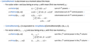
- CentralMoment 也称为关于均值的矩.
- 对于标量阶 r 且 data 为数组
,平均值(第一原始矩)为
: -
![x in TemplateBox[{Vectors, paclet:ref/Vectors}, RefLink, BaseStyle -> {3ColumnTableMod}][n] x in TemplateBox[{Vectors, paclet:ref/Vectors}, RefLink, BaseStyle -> {3ColumnTableMod}][n]](Files/CentralMoment.zh/3.png)

r
次幂之和 »![x in TemplateBox[{Matrices, paclet:ref/Matrices}, RefLink, BaseStyle -> {3ColumnTableMod}][{n,m}] x in TemplateBox[{Matrices, paclet:ref/Matrices}, RefLink, BaseStyle -> {3ColumnTableMod}][{n,m}]](Files/CentralMoment.zh/5.png)

r
次中心幂之纵向和 »![x in TemplateBox[{Arrays, paclet:ref/Arrays}, RefLink, BaseStyle -> {3ColumnTableMod}][{n_(1),...,n_(k)}] x in TemplateBox[{Arrays, paclet:ref/Arrays}, RefLink, BaseStyle -> {3ColumnTableMod}][{n_(1),...,n_(k)}]](Files/CentralMoment.zh/7.png)

r
次中心幂之纵向和 » - CentralMoment[x,r] 等价于 ArrayReduce[CentralMoment[#,r]&,x,1].
- 对于向量阶 {r1,…,rm} 且 data 为数组
,第一原始矩为
: -
![x in TemplateBox[{Matrices, paclet:ref/Matrices}, RefLink, BaseStyle -> {3ColumnTableMod}][{n,m}] x in TemplateBox[{Matrices, paclet:ref/Matrices}, RefLink, BaseStyle -> {3ColumnTableMod}][{n,m}]](Files/CentralMoment.zh/9.png)

第 j 列的 rj
次中心幂之和![x in TemplateBox[{Arrays, paclet:ref/Arrays}, RefLink, BaseStyle -> {3ColumnTableMod}][{n_(1),...,n_(k)}] x in TemplateBox[{Arrays, paclet:ref/Arrays}, RefLink, BaseStyle -> {3ColumnTableMod}][{n_(1),...,n_(k)}]](Files/CentralMoment.zh/11.png)

第 j 列的 rj
次中心幂之和 » - CentralMoment[x,{r1,…,rm}] 等价于 ArrayReduce[CentralMoment[#,
]&,x,{{1},{2}}]. - CentralMoment 能够处理数值型和符号型数据.
- data 还可以有以下形式和解释:
-
Association 值(忽略键值) » WeightedData 加权平均值,基于底层 EmpiricalDistribution » EventData 基于底层 SurvivalDistribution » TimeSeries, TemporalData, … 值的向量或数组(时间戳忽略不计) » Image,Image3D RGB 通道值或灰度强度值 » Audio 所有通道的振幅值 » DateObject, TimeObject 日期列表或时间列表 » - 对于分布 dist,r
阶中心矩由 Expectation[(x-Mean[dist])r,x∈dist] 给出. » - 对于多元分布 dist,{r1,…,rm} 阶中心矩由 Expectation[(x1-μ1)r1⋯(x2-μm)rm,{x1,…,xm}dist] 和 {μ1,…,μm}=Mean[dist] 给出. »
- 对于随机过程 proc,可以计算出时间 t 的切片分布的中心矩函数 SliceDistribution[proc,t],因为
[t]=CentralMoment[SliceDistribution[proc,t],r]. » - CentralMoment[r] 可用于诸如 MomentConvert 和 MomentEvaluate 等函数中.
范例
打开所有单元 关闭所有单元基本范例 (3)
data = RandomVariate[LogNormalDistribution[1, 1], 10 ^ 5];CentralMoment[data, 3]CentralMoment[{Subscript[x, 1], Subscript[x, 2], Subscript[x, 3]}, 2]CentralMoment[{Yesterday, Today, Tomorrow}, 4]CentralMoment[GammaDistribution[α, β], 2]CentralMoment[DirichletDistribution[{Subscript[α, 1], Subscript[α, 2], Subscript[α, 3]}], {1, 1}]范围 (26)
基础用法 (6)
CentralMoment[{1, 2, 3, 4}, 4]CentralMoment[{π, E, 2}, 2]//TogetherCentralMoment[{1., 2., 3., 4.}, 2]CentralMoment[N[{1, 2, 3, 4}, 30], 2]求 WeightedData 的中心矩:
CentralMoment[WeightedData[{1, 2, 3}, {Subscript[w, 1], Subscript[w, 2], Subscript[w, 3]}], 2]data = {8, 3, 5, 4, 9, 0, 4, 2, 2, 3};
weights = {0.15, 0.09, 0.12, 0.10, 0.16, 0., 0.11, 0.08, 0.08, 0.09};CentralMoment[WeightedData[data, weights], 2]求 EventData 的中心矩:
e = {1.0, 2.1, 3.2, 4.5, 5.7};
ci = {0, 0, 0, 1, 0};CentralMoment[EventData[e, ci], 2]求 TimeSeries 的中心矩:
CentralMoment[TemporalData[TimeSeries, {{{2.3, 1.2, 6.7, 5.8, 7.1, 4.6}}, {{0, 5, 1}}, 1, {"Discrete", 1},
{"Discrete", 1}, 1, {}}, False, 10.], 2]CentralMoment[TemporalData[TimeSeries, {{{2.3, 1.2, 6.7, 5.8, 7.1, 4.6}}, {{0, 5, 1}}, 1, {"Discrete", 1},
{"Discrete", 1}, 1, {}}, False, 10.]["Values"], 2]data = Quantity[RandomReal[1, 6], "Meters"]CentralMoment[data, 2]数组数据 (5)
矩阵的 CentralMoment 按列给出矩:
CentralMoment[(| | |
| ----- | ----- |
| a1, 1 | a1, 2 |
| a2, 1 | a2, 2 |), 4]//Simplify张量的 CentralMoment 在第一层按列给出矩:
CentralMoment[Array[Subscript[a, ##]&, {2, 2, 2}], 2]//Simplify//MatrixForm数组的多变量 CentralMoment:
CentralMoment[Array[Subscript[a, ##]&, {2, 2, 2}], {2, 2}]//SimplifyCentralMoment[RandomReal[1, 10 ^ 7], 2]CentralMoment[RandomReal[1, {10 ^ 6, 5}], 2]当输入是 Association 时,CentralMoment 会对其值进行处理:
mat = RandomReal[1, {3, 2}];
assoc = AssociationThread[Range[3], mat]CentralMoment[assoc, 3]SparseArray 数据可以像密集数组一样使用:
CentralMoment[SparseArray[{{1} -> 1, {100} -> 1}], 4]CentralMoment[SparseArray[{{1, 1} -> 1, {2, 2} -> 2, {3, 3} -> 3, {1, 3} -> 4}], 2]求 QuantityArray 的中心矩:
data = QuantityArray[RandomReal[1, 6], "Pounds"]CentralMoment[data, 5]图像和音频数据 (2)
CentralMoment[[image], 5]RGBColor[%]CentralMoment[[image], 4]对于音频对象,CentralMoment 按通道工作:
a = ExampleData[{"Audio", "Bee"}]AudioMeasurements[a, "Channels"]CentralMoment[a, 3]日期和时间 (4)
dates = WolframLanguageData[All, "DateIntroduced"];DateHistogram[dates]CentralMoment[dates, 4]UnitConvert[%, "Decades" ^ 4]dates = RandomDate[4]weights = {1, 1, 1, 3};CentralMoment[WeightedData[dates, weights], 3]UnitConvert[%, "Years" ^ 3]dates = {DateObject[{2024, 2, 29}, CalendarType -> "Julian"], DateObject[{1524, 1, 1}, CalendarType -> "Islamic"], DateObject[{6024, 1, 15}, CalendarType -> "Jewish"]}CentralMoment[dates, 2]UnitConvert[%, "Years" ^ 2]Variance[dates]UnitConvert[%, "Years" ^ 2]RandomTime[3]CentralMoment[%, 4]{TimeObject[{12}, TimeZone -> 0], TimeObject[{12}, TimeZone -> 2], TimeObject[{12}, TimeZone -> "Asia/Tokyo"]}CentralMoment[%, 3]分布与过程矩 (5)
CentralMoment[BinomialDistribution[n, p], 2]//TogetherCentralMoment[NormalDistribution[μ, σ], 2]CentralMoment[BinormalDistribution[{Subscript[μ, 1], Subscript[μ, 2]}, {Subscript[σ, 1], Subscript[σ, 2]}, ρ], 2]CentralMoment[DirichletDistribution[{a, b, c}], 3]CentralMoment[MultinomialDistribution[n, {Subscript[p, 1], Subscript[p, 2], Subscript[p, 3]}], {1, 1, 1}]CentralMoment[BinormalDistribution[{Subscript[μ, 1], Subscript[μ, 2]}, {Subscript[σ, 1], Subscript[σ, 2]}, ρ], {2, 2}]CentralMoment[BetaDistribution[a, b], r]CentralMoment[ExtremeValueDistribution[a, b], r]% /. r -> 3CentralMoment[VonMisesDistribution[Pi / 2, 2], 4]N[%]CentralMoment[TransformedDistribution[x^2, xNormalDistribution[μ, σ]], 2]CentralMoment[ProbabilityDistribution[(Sqrt[2] / π)(1 / (1 + (x - 2)^4)), {x, -∞, ∞}], 2]data = RandomVariate[NormalDistribution[], 10 ^ 3];CentralMoment[HistogramDistribution[data], 4]CentralMoment[BrownianBridgeProcess[μ, σ][t], 4]Plot[Evaluate[% /. {μ -> 3, σ -> 1}], {t, 0, 1}, PlotRange -> All]求 TemporalData 在某时刻 t=0.5 的中心矩:
td = RandomFunction[WienerProcess[1, 1], {0, 10, 0.05}, 100]CentralMoment[td[0.5], 2]Show[ListLinePlot[td, PlotStyle -> Directive[Opacity[0.2], Thin]], Plot[CentralMoment[td[t], 2], {t, 0, 10}, PlotStyle -> Thick]]正式矩 (4)
正式矩的 TraditionalForm 格式:
CentralMoment[r]//TraditionalFormCentralMoment[{p, q, r}]//TraditionalForm将正式矩的组合转换为含 CentralMoment 的表达式:
MomentConvert[Moment[2], CentralMoment]//TraditionalFormMomentConvert[Moment[2]Cumulant[2], CentralMoment]//TraditionalFormMomentEvaluate[CentralMoment[2] + CentralMoment[4], PoissonDistribution[λ]]data = RandomVariate[PoissonDistribution[1], 10^4];MomentEvaluate[CentralMoment[2] + Moment[4], data]求包含 CentralMoment 的一个表达式的样本估计量:
(estimator = MomentConvert[CentralMoment[2], "UnbiasedSampleEstimator"])//TraditionalFormdata = RandomVariate[PoissonDistribution[1], 10^4];MomentEvaluate[estimator, data]应用 (11)
data = RandomReal[{-7, 3}, 100];CentralMoment[data, 1]𝒟 = NormalDistribution[0, σ];CentralMoment[𝒟, 2]Table[Plot[PDF[𝒟, x], {x, -4, 4}, PlotRange -> {0, 0.4}, Filling -> Axis, Ticks -> {Automatic, None}], {σ, {1, 1.5, 2}}]dists = {NormalDistribution[0, 2.5], ChiSquareDistribution[5], GumbelDistribution[3, 2]};Table[CentralMoment[dists[[i]], 3], {i, 3}]//NTable[Plot[PDF[dists[[i]], x], {x, -7, 15}, PlotRange -> {0, 0.2}, Filling -> Axis, Ticks -> {Automatic, None}], {i, 3}]data = RandomVariate[GammaDistribution[3, 6], 10 ^ 4];meq = Table[CentralMoment[data, k] == CentralMoment[GammaDistribution[α, β], k], {k, 2, 3}]NSolve[meq, {α, β}]Show[Histogram[data, Automatic, "ProbabilityDensity"], Plot[Evaluate[PDF[GammaDistribution[α, β], x] /. %], {x, 0, 100}, PlotStyle -> Thick]]使用矩方法,求 GammaDistribution 的正态近似:
gdist = GammaDistribution[α, β];meq = {Moment[gdist, 1] == Moment[NormalDistribution[μ, σ], 1], CentralMoment[gdist, 2] == CentralMoment[NormalDistribution[μ, σ], 2]}Solve[(And@@meq)∧σ > 0, {μ, σ}, Reals]{ndist} = Refine[NormalDistribution[μ, σ] /. %, β > 0∧α > 0]Plot[{PDF[gdist, x], PDF[ndist, x]} /. {α -> 13, β -> 3}, {x, 0, 80}, Evaluated -> True]estim = MomentConvert[CentralMoment[2], "SampleEstimator"]MomentConvert[estim, {CentralMoment, n}]MomentConvert[(estim - %) ^ 2, {CentralMoment, n}]MomentEvaluate[%, UniformDistribution[{0, 1}]]根据大数定理,随样本量增大,样本矩趋近于总体矩. 使用 Histogram 说明在不同样本量时,一个均匀随机变量的二阶样本中心矩的概率分布:
Histogram[Table[CentralMoment[RandomReal[1, {n, 2 * 10 ^ 3}], 2], {n, {10, 10^2, 10^3}}], 30, "ProbabilityDensity", ChartLegends -> {10, 10^2, 10^3}]pdf = (Exp[-(x^2/2)]/Sqrt[2 π]) (1 + ((-6 Sqrt[2] x + 2 Sqrt[2] x^3) CentralMoment[3]/12 Sqrt[2]) + (1/576) (-120 + 360 x^2 - 120 x^4 + 8 x^6) CentralMoment[3]^2 + (1/96) (12 - 24 x^2 + 4 x^4) (-3 + CentralMoment[4]));data = Standardize[Total[RandomReal[1, {3, 10 ^ 5}]]];dist = ProbabilityDistribution[MomentEvaluate[pdf, data], {x, -∞, ∞}]{NExpectation[x ^ 3, xdist], NExpectation[x ^ 4, xdist]}{CentralMoment[data, 3], CentralMoment[data, 4]}Show[Histogram[data, Automatic, "ProbabilityDensity"], Plot[{PDF[dist, z], PDF[NormalDistribution[], z]}, {z, -3, 3}, PlotStyle -> {Directive[Thick], Directive[Dashed, Black]}]]计算样本 Jarque–Bera 统计量的函数 [链接]:
JarqueBera[list_] := With[{cm2 = CentralMoment[list, 2]}, (Length[list]/6)((CentralMoment[list, 3]^2/cm2^3) + (1/4)((CentralMoment[list, 4]/cm2^2) - 3)^2)]data = Table[JarqueBera[RandomVariate[NormalDistribution[], 2 * 10^3]], {2 * 10^3}];Show[
Histogram[data, 30, "ProbabilityDensity"],
Plot[PDF[ChiSquareDistribution[2], x], {x, 0, 20}, PlotRange -> All]]data = TemporalData[TimeSeries, {{{0., 0.007220215826254015, -0.028898335552430553, -0.24236658577144637,
-0.05412788592296647, -0.03667481168713718, -0.17138823136819967, -0.3007558946785308,
-0.43687938826754796, -0.3573927720423709, -0.345586 ... 33201685, -1.2078738741401542, -1.1504147295751919,
-1.1306360665338737}}, {{0, 1., 0.01}}, 1, {"Continuous", 1}, {"Continuous", 1}, 1,
{ValueDimensions -> 1, ResamplingMethod -> {"Interpolation", InterpolationOrder -> 1}}}, False,
10.1];md = MovingMap[CentralMoment[#, 2]&, data, {.1}];ListLinePlot[md, PlotRange -> All]data = RandomFunction[WienerProcess[], {0, 1, .01}, 10 ^ 3];times = Range[0, 1, .1];cm = Map[{#, CentralMoment[data[#], 2]}&, times];Show[ListPlot[data], ListLinePlot[cm, PlotStyle -> Black]]属性和关系 (11)
CentralMoment[ExponentialDistribution[λ], 5]CentralMoment[TransformedDistribution[x + a, xExponentialDistribution[λ]], 5]二阶中心距是一个缩放后的 Variance:
data = RandomReal[10, 20];Variance[data] (Length[data] - 1) / Length[data]CentralMoment[data, 2]CentralMoment[(| | |
| ----- | ----- |
| a1, 1 | a1, 2 |
| a2, 1 | a2, 2 |), 5]//SimplifyCentralMoment[(| | |
| ----- | ----- |
| a1, 1 | a1, 2 |
| a2, 1 | a2, 2 |), {2, 3}]//Simplifyarr = Array[Subscript[a, Row@{##}]&, {n = 4, m = 3, 2, 3}];
rs = {2, 2, 2};
Length[rs] == mCentralMoment[arr, rs] ==
ArrayReduce[Mean,
ArrayReduce[Times@@Power[#, rs]&,
(*Centralize*)
arr - TensorProduct[ConstantArray[1, n], Mean[arr]],
2],
1]//Simplify二阶中心距的 Sqrt 是来自 Mean 的偏差的 RootMeanSquare:
Sqrt[CentralMoment[{a, b, c, d}, 2]]RootMeanSquare[{a, b, c, d} - Mean[{a, b, c, d}]]Skewness 是三阶中心距和二阶中心距的乘方的比:
data = RandomReal[10, 10];Skewness[data]CentralMoment[data, 3] / CentralMoment[data, 2] ^ (3 / 2)Kurtosis 是四阶中心距和二阶中心距的乘方的比:
data = RandomReal[10, 10];Kurtosis[data]CentralMoment[data, 4] / CentralMoment[data, 2] ^ 2CentralMoment 等价于一个随机变量在均值附近的幂的 Expectation:
list = Range[100];Expectation[(x - Mean[list]) ^ 5, xlist] == CentralMoment[list, 5]dist = PoissonDistribution[μ];Expectation[(x - Mean[dist]) ^ 5, xdist] == CentralMoment[dist, 5]阶数为
的 CentralMoment 等价于
,当两者都存在的情况下:
cmgf = CentralMomentGeneratingFunction[LaplaceDistribution[0, 1], t]SeriesCoefficient[cmgf, {t, 0, r}]r!直接使用 CentralMoment:
CentralMoment[LaplaceDistribution[0, 1], r]利用 GeneratingFunction 求中心矩母函数:
GeneratingFunction[CentralMoment[ExponentialDistribution[λ], r] / r!, r, t, Assumptions -> λ > 0]与 CentralMomentGeneratingFunction 的直接计算比较:
CentralMomentGeneratingFunction[ExponentialDistribution[λ], t]FullSimplify[% - %%]CentralMoment 可以使用 Moment、Cumulant 或者 FactorialMoment 表示:
MomentConvert[CentralMoment[4], Cumulant]MomentConvert[CentralMoment[4], Moment]MomentConvert[CentralMoment[2], FactorialMoment]可能存在的问题 (2)
Table[CentralMoment[StudentTDistribution[3], r], {r, 2, 5}]data = RandomVariate[StudentTDistribution[3], {10 ^ 5, 5}];ListLogPlot[Abs@Table[CentralMoment[data, r], {r, 2, 5}], Joined -> True]MomentConvert[CentralMoment[2], "SampleEstimator"]//TraditionalFormMomentConvert[%, {CentralMoment, n}]Limit[%, n -> ∞]MomentConvert[CentralMoment[2], "UnbiasedEstimator", "PowerSymmetricPolynomial"]//TraditionalFormMomentConvert[%, {CentralMoment, n}]巧妙范例 (1)
对 20、100和 300 个样本 CentralMoment 的分布估计:
CentralMoment[ExponentialDistribution[0.9], 2]SmoothHistogram[Table[CentralMoment[RandomVariate[ExponentialDistribution[0.9], {s, 1000}], 2], {s, {20, 100, 300}}], Filling -> Axis, PlotLegends -> {20, 100, 300}, PlotRange -> {{0, 4}, Automatic}]技术笔记
-
▪
- 描述统计
相关指南
-
▪
- 统计矩与母函数 ▪
- 日期和时间 ▪
- 描述性统计分析 ▪
- 符号向量、矩阵和数组
相关的工作流程
- 分析可计算的数据集
文本
Wolfram Research (2007),CentralMoment,Wolfram 语言函数,https://reference.wolfram.com/language/ref/CentralMoment.html (更新于 2024 年).
CMS
Wolfram 语言. 2007. "CentralMoment." Wolfram 语言与系统参考资料中心. Wolfram Research. 最新版本 2024. https://reference.wolfram.com/language/ref/CentralMoment.html.
APA
Wolfram 语言. (2007). CentralMoment. Wolfram 语言与系统参考资料中心. 追溯自 https://reference.wolfram.com/language/ref/CentralMoment.html 年
BibTeX
@misc{reference.wolfram_2026_centralmoment, author="Wolfram Research", title="{CentralMoment}", year="2024", howpublished="\url{https://reference.wolfram.com/language/ref/CentralMoment.html}", note=[Accessed: 19-August-2026]}
BibLaTeX
@online{reference.wolfram_2026_centralmoment, organization={Wolfram Research}, title={CentralMoment}, year={2024}, url={https://reference.wolfram.com/language/ref/CentralMoment.html}, note=[Accessed: 19-August-2026]}