ComplexStreamPlot[f,{z,zmin,zmax}]
ComplexStreamPlot
ComplexStreamPlot[f,{z,zmin,zmax}]
詳細とオプション
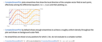
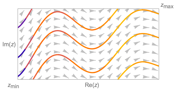
- ComplexStreamPlotは,各点における複素ベクトル場の局所的な方向を示す流線をプロットする.事実上,微分方程式

を解いて
をプロットする. - ComplexStreamPlotは,デフォルトで,プロット全体で密度がほぼ一様となるように十分な数の流線を表示する.背景のスカラー場は表示しない.
- f 等を評価しても複素数にならない位置には流線は表示されない.
- ComplexStreamPlot[f,{z,n}]はComplexStreamPlot[f,{z,-n-n I,n+n I}]に等しい.
- ComplexStreamPlotには属性HoldAllがあり,z に特定の数値を割り当てた後ではじめて f を評価する.場合によっては,まずEvaluate を使って f を記号的に評価した方が効率的かもしれない.
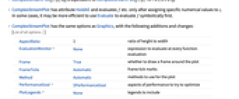
- ComplexStreamPlotにはGraphicsと同じオプションに以下の追加・変更を加えたものが使える. [全オプションのリスト]
-
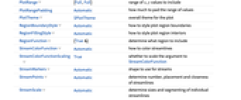
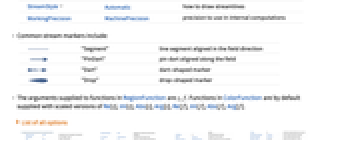
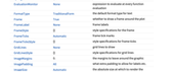
AspectRatio 1 縦横比 EvaluationMonitor None 各関数評価で評価する式 Frame True プロットの周囲に枠を描くかどうか FrameTicks Automatic 枠の目盛マーク Method Automatic プロットに使用するメソッド PerformanceGoal $PerformanceGoal 最適化を試みるパフォーマンスの局面 PlotLegends None 含める凡例 PlotRange {Full,Full} 含める x と y の値の範囲 PlotRangePadding Automatic 値の範囲をどこまで充填するか PlotTheme $PlotTheme プロットの全体的なテーマ RegionBoundaryStyle Automatic プロット領域の境界にどのようにスタイル付けするか RegionFillingStyle Automatic プロット領域の内部にどのようにスタイル付けするか RegionFunction (True&) 含める領域を決定する StreamColorFunction Automatic 流線の彩色方法 StreamColorFunctionScaling True StreamColorFunctionの引数をスケールするかどうか StreamMarkers Automatic 流れに使用する形 StreamPoints Automatic 流線の,数,置き方,近さを決定する StreamScale Automatic 個々の流線の大きさと分割を決定する StreamStyle Automatic 流線の描き方 WorkingPrecision MachinePrecision 内部計算に使われる精度 - 次は,よく使われる流れのマーカーである.
-
"Segment" 場の方向に沿った線分 

"PinDart" 場に沿ったピンダーツ 
"Dart" ダーツの形のマーカー 

"Drop" 滴の形のマーカー - RegionFunction内の関数に渡される引数は,
と
である.ColorFunction内の関数には,デフォルトで,Re[z],Im[z],Abs[z],Arg[z],Re[f],Im[f],Abs[f],Arg[f]のスケールされたバージョンが渡される.
全オプションのリスト
例題
すべて開く すべて閉じる例 (1)
スコープ (22)
サンプリング (8)
Table[ComplexStreamPlot[z^2, {z, -3 - 3I, 3 + 3I}, PlotLabel -> p, StreamPoints -> p], {p, {Coarse, Medium, Automatic, Fine}}]ComplexStreamPlot[z^2, {z, -3 - 3I, 3 + 3I}, StreamPoints -> {1 + I, 1 - I, 2, -2, 2 + 2I, -2 - 2I}]自動シードと明示的なシードの両方を使う.明示的にシードされた流線にはスタイルを付ける:
ComplexStreamPlot[z^2, {z, -3 - 3I, 3 + 3I}, StreamPoints -> {{{1 + I, Red}, {1 - I, Green}, Automatic}}, StreamColorFunction -> None]ComplexStreamPlot[z^2, {z, -3 - 3I, 3 + 3I}, RegionFunction -> Function[{z, f}, Abs[z] < 3]]ComplexStreamPlot[{z^2, Conjugate[z^2]}, {z, -2 - 2I, 2 + 2I}, StreamColorFunction -> None]ComplexStreamPlot[z^2 + 1, {z, -2 - 2I, 2 + 2I}, Mesh -> 5]ComplexStreamPlot[z^2 + 1, {z, -2 - 2I, 2 + 2I}, Mesh -> {{1, 2, 3, 4, 5}}]Evaluateを使って数値割当ての前にベクトル場を記号的に評価する:
ComplexStreamPlot[Evaluate[D[z^3 + z, z]], {z, -2 - 2I, 2 + 2I}]プレゼンテーション (14)
StreamScaleの設定で異なる破線と鏃を指定する:
Table[ComplexStreamPlot[Exp[2z], {z, -2 - 2I, 2 + 2I}, PlotLabel -> ToString@s, StreamScale -> s], {s, {Automatic, None, Full}}]ComplexStreamPlot[Exp[2z], {z, -2 - 2I, 2 + 2I}, StreamColorFunction -> Hue]Table[ComplexStreamPlot[Exp[2z], {z, -2 - 2I, 2 + 2I}, StreamMarkers -> s], {s, {"Toothpick", "Dart", "Drop"}}]ComplexStreamPlot[Exp[2z], {z, -2 - 2I, 2 + 2I}, PlotTheme -> "Business"]ComplexStreamPlot[Exp[2z], {z, -2 - 2I, 2 + 2I}, PlotTheme -> "Business", StreamStyle -> Red, StreamColorFunction -> None]ComplexStreamPlot[Exp[2z], {z, -2 - 2I, 2 + 2I}, StreamColorFunction -> "Rainbow"]ComplexStreamPlot[Exp[2z], {z, -2 - 2I, 2 + 2I}, StreamColorFunction -> None, StreamStyle -> Orange]ComplexStreamPlot[z Exp[2z], {z, -2 - 2I, 2 + 2I}, Mesh -> {{{1, Thick}, {2, Green}, {4, {Thick, Red, Dashed}}}}, MeshStyle -> Opacity[1]]Table[ComplexStreamPlot[z Exp[z], {z, -2 - 2I, 2 + 2I}, Mesh -> 10, MeshStyle -> s], {s, {Red, Thick, Directive[Red, Dashed]}}]ComplexStreamPlot[z Sin[z], {z, -2 - 2I, 2 + 2I}, Mesh -> 10, MeshShading -> {Red, Yellow, Green, None}]regionFn = Function[{z, f}, 4 < Abs[f] < 6 || 0 < Abs[f] < 2];Table[ComplexStreamPlot[z Sin[z], {z, -2 - 2I, 2 + 2I}, RegionFunction -> regionFn, RegionBoundaryStyle -> b], {b, {Red, Thick, Directive[Red, Dashed]}}]ComplexStreamPlot[z Sin[z], {z, -2 - 2I, 2 + 2I}, PlotLegends -> Automatic]ComplexStreamPlot[{z Sin[z], z Cos[z]}, {z, -2 - 2I, 2 + 2I}, PlotLegends -> "Expressions", StreamColorFunction -> None]ComplexStreamPlot[{z Sin[z], z Cos[z]}, {z, -2 - 2I, 2 + 2I}, PlotLegends -> {"first", "second"}, StreamColorFunction -> None]オプション (60)
Background (1)
EvaluationMonitor (2)
PerformanceGoal (2)
PlotLegends (7)
ComplexStreamPlot[Sinc[z], {z, -2 - 2I, 2 + 2I}]ComplexStreamPlot[Sinc[z], {z, -2 - 2I, 2 + 2I}, PlotLegends -> Automatic]ComplexStreamPlot[{Sinc[z], z}, {z, -2 - 2I, 2 + 2I}, PlotLegends -> {"one", "two"}, StreamColorFunction -> None]ComplexStreamPlot[{Sinc[z], z}, {z, -2 - 2I, 2 + 2I}, PlotLegends -> Placed[{"one", "two"}, Below], StreamColorFunction -> None]ComplexStreamPlot[{Sinc[z], z}, {z, -2 - 2I, 2 + 2I}, PlotLegends -> "Expressions", StreamColorFunction -> None]ComplexStreamPlot[{Sinc[z], z}, {z, -2 - 2I, 2 + 2I}, PlotLegends -> Automatic, StreamColorFunction -> None]ComplexStreamPlot[{Sinc[z], z}, {z, -2 - 2I, 2 + 2I}, PlotLegends -> SwatchLegend["Expressions", LegendMarkerSize -> {40, 10}], StreamColorFunction -> None]PlotRange (5)
ComplexStreamPlot[z^3, {z, -2 - 2I, 2 + 2I}, PlotRange -> Full]ComplexStreamPlot[z^3, {z, -2 - 2I, 2 + 2I}, PlotRange -> 1]ComplexStreamPlot[z^3, {z, -2 - 2I, 2 + 2I}, PlotRange -> {{-1, 1}, Automatic}]ComplexStreamPlot[z^3, {z, -2 - 2I, 2 + 2I}, PlotRange -> {Full, {-1, 2}}]ComplexStreamPlot[z^3, {z, -2 - 2I, 2 + 2I}, PlotRange -> {{-2, 1}, {0, 1}}]PlotTheme (3)
ComplexStreamPlot[{Sqrt[z], z^3}, {z, -2 - 2I, 2 + 2I}, PlotTheme -> "Web"]ComplexStreamPlot[{Sqrt[z], z^3}, {z, -2 - 2I, 2 + 2I}, PlotTheme -> "Detailed", StreamColorFunction -> None]ComplexStreamPlot[{Sqrt[z], z^3}, {z, -2 - 2I, 2 + 2I}, PlotTheme -> "Detailed", StreamStyle -> {Red, Blue}, StreamColorFunction -> None]RegionBoundaryStyle (1)
regionFn = Function[{z, f}, n = Norm[z];4 < n < 6 || 0 < n < 2];ComplexStreamPlot[z Sin[z], {z, -2 - 2I, 2 + 2I}, RegionFunction -> regionFn]Table[ComplexStreamPlot[z Sin[z], {z, -2 - 2I, 2 + 2I}, RegionFunction -> regionFn, RegionBoundaryStyle -> b], {b, {Red, Thick, Directive[Red, Dashed]}}]RegionFillingStyle (1)
regionFn = Function[{z, f}, n = Norm[z];4 < n < 6 || 0 < n < 2];ComplexStreamPlot[z Sin[z], {z, -2 - 2I, 2 + 2I}, RegionFunction -> regionFn]ComplexStreamPlot[z Sin[z], {z, -2 - 2I, 2 + 2I}, RegionFunction -> regionFn, RegionFillingStyle -> None]ComplexStreamPlot[z Sin[z], {z, -2 - 2I, 2 + 2I}, RegionFunction -> regionFn, RegionFillingStyle -> Yellow]RegionFunction (3)
ComplexStreamPlot[z^4 + z^2, {z, -2 - 2I, 2 + 2I}, RegionFunction -> Function[{z, f}, Abs[z] < 2]]関数の絶対値が指定された閾値を超えるところにだけ流線をプロットする:
ComplexStreamPlot[z^4 + z^2, {z, -2 - 2I, 2 + 2I}, RegionFunction -> Function[{z, f}, Abs[f] > 2]]ComplexStreamPlot[z^4 + z^2, {z, -2 - 2I, 2 + 2I}, RegionFunction -> Function[{z, f}, Abs[f] < 1 || Abs[f] > 6]]StreamColorFunction (5)
ComplexStreamPlot[z^4 + z^2, {z, -2 - 2I, 2 + 2I}, StreamColorFunction -> Hue]ColorDataから任意の名前付き色勾配を使う:
ComplexStreamPlot[z^4 + z^2, {z, -2 - 2I, 2 + 2I}, StreamColorFunction -> "Rainbow"]定義済みの色勾配用のColorDataを使う:
ComplexStreamPlot[z^4 + z^2, {z, -2 - 2I, 2 + 2I}, StreamColorFunction -> Function[{z, f}, ColorData["AvocadoColors"][Arg[z]]]]ComplexStreamPlot[z^4 + z^2, {z, -2 - 2I, 2 + 2I}, StreamColorFunction -> Function[{z, f}, Blend[{Blue, Red}, Re[z]]]]StreamColorFunctionScalingFalseを使ってスケールされていない値を得る:
ComplexStreamPlot[z^4 + z^2, {z, -2 - 2I, 2 + 2I}, StreamColorFunction -> Hue, StreamColorFunctionScaling -> False]StreamColorFunctionScaling (3)
ComplexStreamPlot[z, {z, -2 - 2I, 2 + 2I}, StreamColorFunction -> Hue]StreamColorFunctionScalingFalseを使ってスケールされていない値を得る:
ComplexStreamPlot[z, {z, -2 - 2I, 2 + 2I}, StreamColorFunction -> Hue, StreamColorFunctionScaling -> False]ComplexStreamPlot[z, {z, -2 - 2I, 2 + 2I}, StreamColorFunction -> Function[{z, f}, Hue[Abs[f], Abs[z], 1]], StreamColorFunctionScaling -> {True, False}]StreamMarkers (8)
ComplexStreamPlot[z^2 - Conjugate[z], {z, -2 - 2I, 2 + 2I}]ComplexStreamPlot[z^2 - Conjugate[z], {z, -2 - 2I, 2 + 2I}, StreamMarkers -> "Drop"]ComplexStreamPlot[{z, z^2 - Conjugate[z]}, {z, -2 - 2I, 2 + 2I}, StreamMarkers -> {"Drop", "Dart"}, StreamColorFunction -> None]Table[ComplexStreamPlot[z^2 Log[z], {z, -2 - 2I, 2 + 2I}, PlotLabel -> s, StreamStyle -> s], {s, {"Segment", "Line"}}]Table[ComplexStreamPlot[z^2 Log[z], {z, -2 - 2I, 2 + 2I}, PlotLabel -> s, StreamScale -> {Full, All, 0.05}, StreamStyle -> s], {s, {"Arrow", "ArrowArrow", "CircleArrow"}}]Table[ComplexStreamPlot[z^2 Log[z], {z, -2 - 2I, 2 + 2I}, PlotLabel -> s, StreamScale -> {Full, All, 0.03}, StreamStyle -> s], {s, {"BarDot", "Dot", "DotArrow", "DotDot"}}]Table[ComplexStreamPlot[z^2 Log[z], {z, -2 - 2I, 2 + 2I}, PlotLabel -> s, StreamScale -> {Full, All, 0.03}, StreamStyle -> s], {s, {"Drop", "BackwardPointer", "Pointer", "Toothpick"}}]Table[ComplexStreamPlot[z^2 Log[z], {z, -2 - 2I, 2 + 2I}, PlotLabel -> s, StreamScale -> {Full, All, 0.03}, StreamStyle -> s], {s, {"Dart", "PinDart", "DoubleDart"}}]StreamPoints (5)
ComplexStreamPlot[z^2 - Conjugate[z], {z, -2 - 2I, 2 + 2I}, StreamPoints -> 10]Table[ComplexStreamPlot[z^2 - Conjugate[z], {z, -2 - 2I, 2 + 2I}, StreamPoints -> p, PlotLabel -> p], {p, {Automatic, Coarse, Fine}}]自動と明示的な両方のシードを使う.明示的にシードした流線にはスタイルを付ける:
ComplexStreamPlot[z^2 - Conjugate[z], {z, -2 - 2I, 2 + 2I}, StreamColorFunction -> None, StreamPoints -> {{{{1, 1}, Red}, {{-1, -1}, Green}, Automatic}}]Table[ComplexStreamPlot[z^2 - Conjugate[z], {z, -2 - 2I, 2 + 2I}, StreamPoints -> {Automatic, d}], {d, {Automatic, 1, Scaled[0.05]}}]Table[ComplexStreamPlot[z^2 - Conjugate[z], {z, -2 - 2I, 2 + 2I}, StreamPoints -> {Automatic, d}], {d, {Automatic, {Scaled[0.1], Scaled[0.5]}}}]StreamScale (9)
ComplexStreamPlot[z^3 - Conjugate[z], {z, -2 - 2I, 2 + 2I}, StreamScale -> Full]ComplexStreamPlot[z^3 - Conjugate[z], {z, -2 - 2I, 2 + 2I}, StreamScale -> None]Table[ComplexStreamPlot[z^3 - Conjugate[z], {z, -2 - 2I, 2 + 2I}, PlotLabel -> s, StreamScale -> s], {s, {Tiny, Large}}]Table[ComplexStreamPlot[z^3 - Conjugate[z], {z, -2 - 2I, 2 + 2I}, PlotLabel -> s, StreamScale -> s], {s, {0.1, 0.2, 0.4}}]ComplexStreamPlot[z^3 - Conjugate[z], {z, -2 - 2I, 2 + 2I}, StreamScale -> {{0.1, 0.1}, Automatic}]Table[ComplexStreamPlot[z^3 - Conjugate[z], {z, -2 - 2I, 2 + 2I}, PlotLabel -> n, StreamScale -> {Full, n}], {n, {12, 24, All}}]Table[ComplexStreamPlot[z^3 - Conjugate[z], {z, -2 - 2I, 2 + 2I}, PlotLabel -> a, StreamScale -> {Automatic, Automatic, a}], {a, {.02, .04}}]Table[ComplexStreamPlot[z^3 - Conjugate[z], {z, -2 - 2I, 2 + 2I}, PlotLabel -> a, StreamScale -> {Automatic, Automatic, a}], {a, {Scaled[0.5], Scaled[1], Scaled[1.5]}}]ComplexStreamPlot[z^3 - Conjugate[z], {z, -2 - 2I, 2 + 2I}, StreamScale -> {Automatic, 2, Automatic, Function[{z, f}, Re[z]]}]StreamStyle (5)
StreamColorFunctionは,色についてはStreamStyleより優先される:
ComplexStreamPlot[z^2 Log[z], {z, -2 - 2I, 2 + 2I}, StreamStyle -> Red]StreamColorFunctionNoneを使ってStreamStyleで色を指定する:
ComplexStreamPlot[z^2 Log[z], {z, -2 - 2I, 2 + 2I}, StreamStyle -> Red, StreamColorFunction -> None]Table[ComplexStreamPlot[z^2 Log[z], {z, -2 - 2I, 2 + 2I}, StreamStyle -> s, StreamColorFunction -> None], {s, {Orange, Thick, Directive[Orange, Dashed]}}]ComplexStreamPlot[z^2 Log[z], {z, -2 - 2I, 2 + 2I}, StreamScale -> Full, StreamStyle -> Arrowheads[{{0.03, Automatic, Graphics[Circle[]]}}]]ComplexStreamPlot[{z, z^2 Log[z]}, {z, -2 - 2I, 2 + 2I}, StreamStyle -> {Red, Blue}, StreamColorFunction -> None]アプリケーション (10)
基本的なアプリケーション (1)
ComplexStreamPlot[z, {z, 5}]ComplexStreamPlot[z + 1, {z, 5}]ComplexStreamPlot[z ^ 2, {z, 5}]ComplexStreamPlot[Sqrt[z], {z, 5}]ComplexStreamPlot[Sin[z], {z, 5}]ComplexStreamPlot[Log[z], {z, 5}]ComplexStreamPlot[1 / z, {z, 5}]ComplexStreamPlot[1 / z ^ 2, {z, 5}]その他のアプリケーション (9)
ComplexStreamPlot[z, {z, -3 - 3I, 3 + 3I}]ComplexStreamPlot[-z, {z, -3 - 3I, 3 + 3I}]
のとき,複素関数
に対応する実ベクトル場は
であり,場に従う軌跡は微分方程式
を満足する.陰的な解は実数
について
であるが,これは原点における実軸に接する円の族に対応する:
Show[ContourPlot[(x^2/y) + y, {x, -3, 3}, {y, -3, 3}, ContourShading -> None, ContourStyle -> Red, Contours -> Range[-8, 8]], ComplexStreamPlot[z^2, {z, -3 - 3I, 3 + 3I}, StreamColorFunction -> None]]Show[PolarPlot[Evaluate@Table[c Sin[θ], {c, -3, 3}], {θ, 0, π}, PlotStyle -> Red], ComplexStreamPlot[z^2, {z, -3 - 3I, 3 + 3I}, StreamColorFunction -> None]]より一般的には,
が整数である
について,流線は定数
について
に従う:
n = 4;Show[PolarPlot[Evaluate@Table[c Surd[Sin[(n - 1)θ], n - 1], {c, -3, 3}], {θ, 0, π}, PlotStyle -> Red], ComplexStreamPlot[z^n, {z, -3 - 3I, 3 + 3I}, StreamColorFunction -> None]]n = -4;Show[PolarPlot[Evaluate@Table[c Surd[Sin[(n - 1)θ], n - 1], {c, -3, 3}], {θ, 0, π}, PlotStyle -> Red], ComplexStreamPlot[z^n, {z, -3 - 3I, 3 + 3I}, StreamColorFunction -> None], PlotRange -> 3]次数が
で零点近くでは,流線は
方向で零点から始まって零点で終るループを形成する:
n = 3;Show[ComplexPlot[z^n, {z, -3 - 3I, 3 + 3I}, ColorFunction -> None], ComplexStreamPlot[z^n, {z, -3 - 3I, 3 + 3I}, StreamStyle -> White, StreamColorFunction -> None, StreamScale -> Large]]次数
の極近くでは,流線は
方向から極に収束し,
方向から極から発散する:
n = 2;Show[ComplexPlot[1 / z^n, {z, -3 - 3I, 3 + 3I}, ColorFunction -> None], ComplexStreamPlot[1 / z^n, {z, -3 - 3I, 3 + 3I}, StreamStyle -> White, StreamColorFunction -> None, StreamScale -> Large]]ComplexStreamPlot[(z^2 + 2 z - 3/z^4 - 6 z^3 + 18 z^2 - 54 z + 81), {z, -5 - 5I, 5 + 5I}]ComplexStreamPlot[Exp[-5 / z], {z, -1 - I, 1 + I}]ComplexStreamPlot[#, {z, -1 - I, 1 + I}]& /@ NestList[D[#, z]&, z^3, 3]ComplexStreamPlot[Conjugate[z^2], {z, -2 - 2I, 2 + 2I}]
は理想流体の流れについての複素ポテンシャルであるとすると,
は速度ポテンシャル,
は流線関数であり,流体速度場は
となる.コーシー・リーマン(Cauchy–Riemann)方程式により,
であるので,
の共役で流線プロットが生成できる.循環するシリンダーの周りの流れの流線を表示する:
F = z + (1/z) + I Log[z];ComplexStreamPlot[Evaluate[Conjugate[D[F, z]]], {z, -2 - 2I, 2 + 2I}, Epilog -> {Circle[]}, StreamScale -> Full, StreamStyle -> "Line"]F = (-I z)^2 / 3 - (-z)^2 / 3;ComplexStreamPlot[Evaluate[Conjugate[D[F, z]]], {z, -2 - 2I, 2 + 2I}, StreamScale -> Full, StreamStyle -> "Line", RegionFunction -> Function[{z, f}, Arg[z] < -π / 2 || Arg[z] > 0]]特性と関係 (15)
ComplexStreamPlotはStreamPlotの特殊ケースである:
{ComplexStreamPlot[Sin[z], {z, 4}], StreamPlot[ReIm[Sin[x + I * y]], {x, -4 , 4}, {y, -4, 4}]}ComplexVectorPlotは複素数をベクトルとしてプロットする:
ComplexVectorPlot[Log[z], {z, 3}]ComplexVectorPlotはVectorPlotの特殊ケースである:
VectorPlot[ReIm[Log[x + I y]], {x, -3, 3}, {y, -3, 3}]VectorDisplacementPlotを使って複素関数の指定領域に対する影響を可視化する:
VectorDisplacementPlot[ReIm[Sin[x + I y]], {x, y}∈Annulus[], VectorPoints -> Automatic, VectorSizes -> Full]VectorPlot3DとStreamPlot3Dを使って3Dベクトル場を可視化する:
{VectorPlot3D[{z, x, y}, {x, -1, 1}, {y, -1, 1}, {z, -1, 1}], StreamPlot3D[{z, x, y}, {x, -1, 1}, {y, -1, 1}, {z, -1, 1}]}ComplexContourPlotは複素数上に曲線をプロットする:
ComplexContourPlot[Abs[Log[z]] == 1, {z, 3}]ComplexRegionPlotは複素数上に領域をプロットする:
ComplexRegionPlot[Abs[Log[z]] < 1, {z, 3}]ComplexPlotは関数の引数と大きさを色を使って示す:
ComplexPlot[Log[z], {z, 3}]ComplexPlot3Dを使って
軸を大きさに使う:
ComplexPlot3D[Log[z], {z, 3}]複素数の配列にComplexArrayPlotを使う:
ComplexArrayPlot[Table[x ^ 3 + I y ^ 2, {x, -2, 2, 0.1}, {y, -2, 2, 0.1}]]ReImPlotとAbsArgPlotを使って複素数値を実数上にプロットする:
ReImPlot[Log[x], {x, -3, 3}]AbsArgPlot[Log[x], {x, -3, 3}]ComplexListPlotを使って複素数の位置を平面上に示す:
ComplexListPlot[RandomComplex[{-3 - 3I, 3 + 3I}, 100]]ListVectorPlotをデータのプロットに使う:
data = Table[ReIm[(x + I y)^2], {x, -3, 3, 0.2}, {y, -3, 3, 0.2}];ListVectorPlot[data]ListStreamPlotを使ってベクトルの代りに流れをプロットする:
ListStreamPlot[data]VectorDensityPlotを使ってスカラー場の密度プロットを加える:
VectorDensityPlot[ReIm[(x + I y)^2], {x, -3, 3}, {y, -3, 3}]StreamDensityPlotを使ってベクトルの代りに流れを使う:
StreamDensityPlot[ReIm[(x + I y)^2], {x, -3, 3}, {y, -3, 3}]ListVectorDensityPlotを使ってスカラー場の密度プロットをデータに基づいて生成する:
data = Table[{{x, y}, ReIm[(x + I y)^2 + 1]}, {x, -3, 3, 0.2}, {y, -3, 3, 0.2}];ListVectorDensityPlot[data]ListStreamDensityPlotを使ってベクトルの代りに流れをプロットする:
ListStreamDensityPlot[data]LineIntegralConvolutionPlotを使ってベクトル場の線積分のたたみ込みをプロットする:
LineIntegralConvolutionPlot[ReIm[(x + I y)^3], {x, -3, 3}, {y, -3, 3}]テキスト
Wolfram Research (2020), ComplexStreamPlot, Wolfram言語関数, https://reference.wolfram.com/language/ref/ComplexStreamPlot.html (2020年に更新).
CMS
Wolfram Language. 2020. "ComplexStreamPlot." Wolfram Language & System Documentation Center. Wolfram Research. Last Modified 2020. https://reference.wolfram.com/language/ref/ComplexStreamPlot.html.
APA
Wolfram Language. (2020). ComplexStreamPlot. Wolfram Language & System Documentation Center. Retrieved from https://reference.wolfram.com/language/ref/ComplexStreamPlot.html
BibTeX
@misc{reference.wolfram_2026_complexstreamplot, author="Wolfram Research", title="{ComplexStreamPlot}", year="2020", howpublished="\url{https://reference.wolfram.com/language/ref/ComplexStreamPlot.html}", note=[Accessed: 11-September-2026]}
BibLaTeX
@online{reference.wolfram_2026_complexstreamplot, organization={Wolfram Research}, title={ComplexStreamPlot}, year={2020}, url={https://reference.wolfram.com/language/ref/ComplexStreamPlot.html}, note=[Accessed: 11-September-2026]}