


ComplexArrayPlot
ComplexArrayPlot[array]
generates a plot in which complex values zij in an array array are shown in a discrete array of squares with Arg[zij] indicated by color and Abs[zij] by shading.
Details and Options
- ComplexArrayPlot is used to visualize tables of complex numbers.
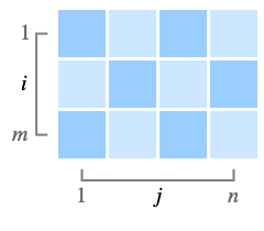
- ComplexArrayPlot[array] by default arranges successive rows of the mn dimensional array down the page and successive columns across, just as a table or grid would normally be formatted.
- ComplexArrayPlot uses a cyclic color function over the values of Arg[zij] and shading to indicate values of Abs[zij]. Complex numbers with large moduli are lighter than numbers with smaller moduli.
- In ComplexArrayPlot[array], array can have the following forms:
-
{{z11,z12,…,z1n},…,{zm1,zm2,…,zmn}} values zij SparseArray values as a normal array NumericArray values as a normal array Dataset values as a normal array - The following special entries can be used for the zij:
-
None background color color directive specified color - If array is ragged, shorter rows are treated as padded on the right with background.
- ComplexArrayPlot has the same options as Graphics, with the following additions and changes: [List of all options]
-
AspectRatio Automatic ratio of height to width ClippingStyle None how to show cells whose values are clipped ColorFunction Automatic how each cell should be colored ColorFunctionScaling True whether to scale the argument to ColorFunction ColorRules Automatic rules for determining colors from values DataRange All the range of  and
and  values to assume
 DataReversed False whether to reverse the order of rows Frame Automatic whether to draw a frame around the plot FrameLabel None labels for rows and columns FrameTicks None what ticks to include on the frame MaxPlotPoints Infinity the maximum number of points to include Mesh False whether to draw a mesh MeshStyle GrayLevel[GoldenRatio-1] the style to use for a mesh PerformanceGoal $PerformanceGoal aspects of performance to try to optimize PlotLegends None legends for datasets PlotRange All the range of values to plot PlotTheme $PlotTheme overall theme for the plot TargetUnits Automatic units to display in the plot - The rules given by ColorRules are applied to the value
 of each cell. The rules can involve patterns.
 - If none of the rules in ColorRules apply, then ColorFunction is used to determine the color.
- With the default setting ColorRules->Automatic, an explicit setting ColorFunctioncfunc is used instead of ColorRules.
- ColorFunction->{cfunc,sfunc} uses cfunc to generate the base color and sfunc to adjust the color to highlight features.
- Possible named settings for sfunc are:
-
Automatic automatic shading based on Abs[z] 
"MaxAbs" light shading of large values of Abs[z] 
"LocalMaxAbs" light shading of an upper quantile of Abs[z] 
"GlobalAbs" dark to light shading of small to large values of Abs[z] 
"QuantileAbs" dark to light shading based on quantiles of Abs[z] 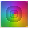
"CyclicLogAbs" cyclic dark to light shading of Log[Abs[z]] 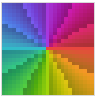
"CyclicArg" cyclic dark to light shading of Arg[z] 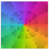
"CyclicLogAbsArg" cyclic shading of Log[Abs[z]] and Arg[z] 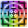
"CyclicReImLogAbs" dark cycles of Re[z] and Im[z] and light cycles of Log[Abs[z]] 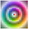
"ShiftedCyclicLogAbs" cyclic shading of Log[Abs[z]] after a threshold 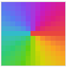
None no shading - Functions in ColorFunction are by default supplied with scaled versions of Re[z], Im[z], Abs[z], Arg[z].
- If the color determined for a particular cell is None, the cell is rendered in the background color.
- If no color is determined for a particular cell, the cell is rendered in a default dark red color.
- With DataReversed->True, the order of rows is reversed, so that rows run from bottom to top, with the last row at the top.
- With the setting FrameTicks->Automatic, ticks are placed at round integers, typically multiples of 5 or 10.
- With the setting FrameTicks->All, ticks are also placed at the minimum and maximum
 and
and  .
. - In explicit FrameTicks specifications, the tick coordinates are taken to refer to
 and
and  .
. - PlotRange can take the following forms:
-
zmax show Abs[zij] values between 0 and zmax {zmin,zmax} show Abs[zij] values between zmin and zmax {rangei,rangej} show zij values with i in rangei and j in rangej {rangei,rangej,rangez} show zij values with i in rangei, j in rangej, and zij in rangez - The array index ranges rangei and rangej can take the following forms:
-
{min,max} include indices between min and max All include all indices - Typical settings for PlotLegends include:
-
None no legend Automatic automatically determine legend Placed[lspec,…] specify placement for legend - Mesh->True draws mesh lines between each cell in the array.
- Mesh->{mi,mj} gives mesh specifications for the
 and
and  directions, respectively.
 - With the default setting Frame->Automatic, a frame is drawn only when Mesh->False.
- For purposes of combining with other graphics, the array element
 is taken to cover a unit square centered at coordinate position
  ,
,  .
. - A setting DataRange->{{xmin,xmax},{ymin,ymax}} specifies that the centers of successive cells should be at equally spaced positions between xmin and xmax in the horizontal direction, and ymin and ymax in the vertical direction. With the default setting DataReversed->False,
 is centered at {xmin,ymax}.
 - With the default setting DataRange->All and DataReversed->False, the array element
 will be taken to cover a unit square centered at coordinate position
  ,
,  .
. -
AlignmentPoint Center the default point in the graphic to align with AspectRatio Automatic ratio of height to width Axes False whether to draw axes AxesLabel None axes labels AxesOrigin Automatic where axes should cross AxesStyle {} style specifications for the axes Background None background color for the plot BaselinePosition Automatic how to align with a surrounding text baseline BaseStyle {} base style specifications for the graphic ClippingStyle None how to show cells whose values are clipped ColorFunction Automatic how each cell should be colored ColorFunctionScaling True whether to scale the argument to ColorFunction ColorRules Automatic rules for determining colors from values ContentSelectable Automatic whether to allow contents to be selected CoordinatesToolOptions Automatic detailed behavior of the coordinates tool DataRange All the range of  and
and  values to assume
 DataReversed False whether to reverse the order of rows Epilog {} primitives rendered after the main plot FormatType TraditionalForm the default format type for text Frame Automatic whether to draw a frame around the plot FrameLabel None labels for rows and columns FrameStyle {} style specifications for the frame FrameTicks None what ticks to include on the frame FrameTicksStyle {} style specifications for frame ticks GridLines None grid lines to draw GridLinesStyle {} style specifications for grid lines ImageMargins 0. the margins to leave around the graphic ImagePadding All what extra padding to allow for labels etc. ImageSize Automatic the absolute size at which to render the graphic LabelStyle {} style specifications for labels MaxPlotPoints Infinity the maximum number of points to include Mesh False whether to draw a mesh MeshStyle GrayLevel[GoldenRatio-1] the style to use for a mesh Method Automatic details of graphics methods to use PerformanceGoal $PerformanceGoal aspects of performance to try to optimize PlotLabel None an overall label for the plot PlotLegends None legends for datasets PlotRange All the range of values to plot PlotRangeClipping False whether to clip at the plot range PlotRangePadding Automatic how much to pad the range of values PlotRegion Automatic the final display region to be filled PlotTheme $PlotTheme overall theme for the plot PreserveImageOptions Automatic whether to preserve image options when displaying new versions of the same graphic Prolog {} primitives rendered before the main plot RotateLabel True whether to rotate y labels on the frame TargetUnits Automatic units to display in the plot Ticks Automatic axes ticks TicksStyle {} style specifications for axes ticks
List of all options
Examples
open all close allBasic Examples (3)
ComplexArrayPlot[{{I, 1 + I, 1 - I}, {1, I / 2, 2 + 3I}}]Give explicit color directives to specify colors for individual cells:
ComplexArrayPlot[{{Gray, Orange, 1 - I}, {1, I / 2, 2 + 3I}}]ComplexArrayPlot[RandomComplex[{-1 - I, 1 + I}, {10, 20}]]Scope (14)
Data (8)
By default, colors change with argument from ![]() (cyan) to
(cyan) to ![]() (red) to
(red) to ![]() (cyan):
(cyan):
ComplexArrayPlot[{{-1 + I, I, 1 + I}, {-1, 0, 1}, {-1 - I, -I, 1 - I}}]By default, colors are lighter for complex numbers with larger moduli:
ComplexArrayPlot[{{-2 + 2 I, -1 + 2 I, 2 I, 1 + 2 I, 2 + 2 I}, {-2 + I, -1 + I, I, 1 + I, 2 + I}, {-2, -1, 0, 1, 2}, {-2 - I, -1 - I, -I, 1 - I, 2 - I}, {-2 - 2 I, -1 - 2 I, -2 I, 1 - 2 I, 2 - 2 I}}]Unknown, symbolic or missing values are shown dark red:
ComplexArrayPlot[{{X, Y, Z }, {, 0, 1}, {-1 - I, -I, Null}}]Specify explicit colors for cells:
ComplexArrayPlot[{{Red, I, 1 + I}, {-1, Green, 1}, {-1 - I, -I, Blue}}]Plot a ragged array, padding on the right:
ComplexArrayPlot[{{-1 + I}, {-1, 0}, {-1 - I, -I, 1 - I}}]Cells with value None are rendered like the background:
ComplexArrayPlot[{{-1 + I, None, 1 + I}, {-1, None, 1}, {-1 - I, None, 1 - I}}]ComplexArrayPlot[SparseArray[{{x_, x_} -> 1 + I, ({x_, y_} /; Abs[x - y] < 3) :> RandomComplex[{-1 - I, 1 + I}]}, {10, 10}]]ComplexArrayPlot[RawArray["Complex64", {{-4.005686283111572 + 3.604153871536255*I,
4.635770320892334 - 1.1016300916671753*I, 1.9577208757400513 + 4.972633361816406*I,
3.506197690963745 - 0.33499598503112793*I, -2.474790334701538 - 3.884897232055664*I,
1 ... 9864978790283*I,
1.6527553796768188 + 0.20232297480106354*I, -1.0656682252883911 + 0.8207247257232666*I,
-1.9840965270996094 - 1.6973134279251099*I, 3.3480541706085205 - 4.883756160736084*I,
-4.373885631561279 + 2.1675751209259033*I}}]]Presentation (6)
ComplexArrayPlot[{{-1 + I, I, 1 + I}, {-1, 0, 1}, {-1 - I, -I, 1 - I}}, Mesh -> True]ComplexArrayPlot[Reverse@Table[real + I imag, {imag, -10, 10}, {real, -10, 10}], PlotLegends -> Automatic]ComplexArrayPlot[Reverse@Table[real + I imag, {imag, -10, 10}, {real, -10, 10}], PlotLegends -> Automatic, ColorFunction -> {Automatic, None}]ComplexArrayPlot[Reverse@Table[real + I imag, {imag, -10, 10}, {real, -10, 10}], ColorFunction -> {"WatermelonColors", None}]Use shading schemes like ComplexPlot:
ComplexArrayPlot[Reverse@Table[real + I imag, {imag, -40, 40}, {real, -40, 40}], ColorFunction -> "ShiftedCyclicLogAbs"]Choose a color function and a shading scheme:
ComplexArrayPlot[Reverse@Table[real + I imag, {imag, -40, 40}, {real, -40, 40}], ColorFunction -> {"WatermelonColors", "ShiftedCyclicLogAbs"}]Options (71)
AspectRatio (4)
By default, the ratio of the height to width for the plot is determined automatically:
ComplexArrayPlot[Mod[Array[Binomial, {32, 32}, 0], 1 + I]]Use numerical value to specify the height to width ratio:
ComplexArrayPlot[Mod[Array[Binomial, {32, 32}, 0], 1 + I], AspectRatio -> 1 / 2]Make the height the same as the width with AspectRatio1:
ComplexArrayPlot[Mod[Array[Binomial, {32, 32}, 0], 1 + I], AspectRatio -> 1]AspectRatioFull adjusts the height and width to tightly fit inside other constructs:
plot = ComplexArrayPlot[Mod[Array[Binomial, {32, 32}, 0], 1 + I], AspectRatio -> Full];{Framed[Pane[plot, {50, 100}]], Framed[Pane[plot, {100, 100}]], Framed[Pane[plot, {100, 50}]]}Axes (4)
By default, ComplexArrayPlot uses a frame instead of axes:
ComplexArrayPlot[Mod[Array[Binomial, {32, 32}, 0], 1 + I]]ComplexArrayPlot[Mod[Array[Binomial, {32, 32}, 0], 1 + I], Frame -> False, Axes -> True]Use AxesOrigin to specify where the axes intersect:
ComplexArrayPlot[Mod[Array[Binomial, {32, 32}, 0], 1 + I], Frame -> False, Axes -> True, AxesOrigin -> {0, 0}]Turn each axis on individually:
{ComplexArrayPlot[Mod[Array[Binomial, {32, 32}, 0], 1 + I], Frame -> False, Axes -> {True, False}], ComplexArrayPlot[Mod[Array[Binomial, {32, 32}, 0], 1 + I], Frame -> False, Axes -> {False, True}]}AxesLabel (3)
No axes labels are drawn by default:
ComplexArrayPlot[Mod[Array[Binomial, {32, 32}, 0], 1 + I], Frame -> False, Axes -> True]ComplexArrayPlot[Mod[Array[Binomial, {32, 32}, 0], 1 + I], Frame -> False, Axes -> True, AxesLabel -> "Label"]ComplexArrayPlot[Mod[Array[Binomial, {32, 32}, 0], 1 + I], Frame -> False, Axes -> True, AxesLabel -> {"label 1", "Label 2"}]AxesOrigin (2)
The position of the axes is determined automatically:
ComplexArrayPlot[Mod[Array[Binomial, {32, 32}, 0], 1 + I], Frame -> False, Axes -> True, AxesOrigin -> Automatic]Specify an explicit origin for the axes:
ComplexArrayPlot[Mod[Array[Binomial, {32, 32}, 0], 1 + I], Frame -> False, Axes -> True, AxesOrigin -> {25, 25}]AxesStyle (4)
ComplexArrayPlot[Mod[Array[Binomial, {32, 32}, 0], 1 + I], Frame -> False, Axes -> True, AxesStyle -> Red]Specify a style for each axis:
ComplexArrayPlot[Mod[Array[Binomial, {32, 32}, 0], 1 + I], Frame -> False, Axes -> True, AxesStyle -> {{Thick, Red}, {Thick, Blue}}]Use different styles for the ticks and the axes:
ComplexArrayPlot[Mod[Array[Binomial, {32, 32}, 0], 1 + I], Frame -> False, Axes -> True, AxesStyle -> Green, TicksStyle -> StandardBlue]Use different styles for the labels and the axes:
ComplexArrayPlot[Mod[Array[Binomial, {32, 32}, 0], 1 + I], Frame -> False, Axes -> True, AxesStyle -> Green, LabelStyle -> StandardBlue]Background (4)
Background is normally visible only around the edges:
ComplexArrayPlot[{{0, 1, 2, 3}, {I, 1 + I, 2 + I, 3 + I}, {2 I, 1 + 2 I, 2 + 2 I, 3 + 2 I}}, Background -> Blue]The background "shows through" whenever an explicit entry is None:
ComplexArrayPlot[{{None, 1, 2, 3}, {I, None, 2 + I, 3 + I}, {2 I, 1 + 2 I, None, 3 + 2 I}}, Background -> Blue]Background also by default shows through for values outside the plot range:
ComplexArrayPlot[{{0, 1, 2, 3}, {I, 1 + I, 2 + I, 3 + I}, {2 I, 1 + 2 I, 2 + 2 I, 3 + 2 I}}, Background -> Blue, PlotRange -> {1, 3}]ClippingStyle overrides background color:
ComplexArrayPlot[{{0, 1, 2, 3}, {I, 1 + I, 2 + I, 3 + I}, {2 I, 1 + 2 I, 2 + 2 I, 3 + 2 I}}, Background -> Blue, PlotRange -> {1, 3}, ClippingStyle -> {White, Black}]ClippingStyle (3)
The default is to show values of ![]() with values outside the
with values outside the ![]() plot range in the background color:
plot range in the background color:
ComplexArrayPlot[Table[(real + I imag)^2 + 1, {imag, -5, 5}, {real, -5, 5}], PlotRange -> {3, 20}]Show values outside the plot range in red:
ComplexArrayPlot[Table[(real + I imag)^2 + 1, {imag, -5, 5}, {real, -5, 5}], PlotRange -> {3, 20}, ClippingStyle -> Red]Show low values in black and high values in red:
ComplexArrayPlot[Table[(real + I imag)^2 + 1, {imag, -5, 5}, {real, -5, 5}], PlotRange -> {3, 20}, ClippingStyle -> {Black, Red}]ColorFunction (9)
By default, complex ![]() values are colored by Arg[z] and shaded by Abs[z]:
values are colored by Arg[z] and shaded by Abs[z]:
ComplexArrayPlot[Table[(real + I imag)^4 + 1, {imag, -20, 20}, {real, -20, 20}]]Turn off the shading based on Abs[z]:
ComplexArrayPlot[Table[(real + I imag)^4 + 1, {imag, -20, 20}, {real, -20, 20}], ColorFunction -> None]Map modulus values from 0 to 1 onto colors according to Hue:
ComplexArrayPlot[Table[(real + I imag)^4 + 1, {imag, -20, 20}, {real, -20, 20}], ColorFunction -> Hue]Use a pure function as the color function:
ComplexArrayPlot[Table[(real + I imag)^4 + 1, {imag, -20, 20}, {real, -20, 20}], ColorFunction -> (GrayLevel[#4]&)]Use a named color gradient from ColorData:
ComplexArrayPlot[Table[(real + I imag)^4 + 1, {imag, -20, 20}, {real, -20, 20}], ColorFunction -> "StarryNightColors"]ComplexArrayPlot[Table[(real + I imag)^4 + 1, {imag, -50, 50}, {real, -50, 50}], ColorFunction -> "ShiftedCyclicLogAbs"]Specify a color function and a shading scheme:
ComplexArrayPlot[Table[(real + I imag)^4 + 1, {imag, -50, 50}, {real, -50, 50}], ColorFunction -> {"DarkRainbow", "CyclicArg"}]With ColorFunctionScalingTrue, the values are first scaled to lie between 0 and 1:
ComplexArrayPlot[Table[(real + I imag)^4 + 1, {imag, -50, 50}, {real, -50, 50}], ColorFunction -> "DarkRainbow", ColorFunctionScaling -> False]Use a color function that colors complex values ![]() by Re[z], Im[z], Abs[z] or Arg[z]:
by Re[z], Im[z], Abs[z] or Arg[z]:
ComplexArrayPlot[Table[(real + I imag)^4 + 1, {imag, -50, 50}, {real, -50, 50}], ColorFunction -> Function[{re, im, abs, arg}, Blend[{Red, Green}, abs]]]ColorFunctionScaling (3)
By default, values are scaled to lie between 0 to 1 before applying the color function:
ComplexArrayPlot[Table[(real + I imag)^4 + 1, {imag, -20, 20}, {real, -20, 20}], ColorFunctionScaling -> True, PlotLegends -> Automatic]Choose to not scale the argument prior to applying the color function:
ComplexArrayPlot[Table[(real + I imag)^4 + 1, {imag, -20, 20}, {real, -20, 20}], ColorFunctionScaling -> False, PlotLegends -> Automatic]Some color functions are not cyclic so the colors only change in a small band:
ComplexArrayPlot[Table[(real + I imag)^4 + 1, {imag, -50, 50}, {real, -50, 50}], ColorFunction -> "DarkRainbow", ColorFunctionScaling -> False, PlotLegends -> Automatic]ColorRules (6)
Specify color rules for explicit values:
ComplexArrayPlot[Table[Gamma[real + I imag], {imag, -5, 5}, {real, -5, 5}], ColorRules -> {1 -> Black, Gamma[3I] -> White, Gamma[-3I] -> White}]Specify color rules for patterns:
realQ[z_] := Re[z] == zComplexArrayPlot[Table[Gamma[real + I imag], {imag, -5, 5}, {real, -5, 5}], ColorRules -> {_ ? realQ -> Black}]ColorFunction is used if no color rules apply:
imaginaryQ[z_] := I Im[z] == zComplexArrayPlot[Table[Gamma[real + I imag], {imag, -5, 5}, {real, -5, 5}], ColorRules -> {_ ? imaginaryQ -> Black}]The array can contain symbolic values:
ComplexArrayPlot[Transpose[Permutations[{a, b, c}]], ColorRules -> {a -> Red, b -> Yellow, c -> Blue}, Mesh -> True]Implement a "default color" by adding a rule for _:
realQ[z_] := Re[z] == zComplexArrayPlot[Table[Gamma[real + I imag], {imag, -2, 2}, {real, -2, 2}], ColorRules -> {_ ? realQ -> Black, _ -> Yellow}]Rules are used in the order given:
realQ[z_] := Re[z] == zComplexArrayPlot[Table[Gamma[real + I imag], {imag, -5, 5}, {real, -5, 5}], ColorRules -> {1 -> White, _ ? realQ -> Black}]DataRange (5)
By default, data is plotted at integer coordinates:
ComplexArrayPlot[Table[Gamma[real + I imag], {imag, 0, 3}, {real, 0, 5}], FrameTicks -> Automatic]ComplexArrayPlot[Table[Gamma[real + I imag], {imag, 0, 3}, {real, 0, 5}], FrameTicks -> Automatic, DataRange -> {{0, 5}, {0, 3}}]Specify a range for the data with a pair of complex numbers:
ComplexArrayPlot[Table[Gamma[real + I imag], {imag, 0, 3}, {real, 0, 5}], FrameTicks -> Automatic, DataRange -> {1 + 2I, 6 + 5I}]Specify the bottom-left corner of the data range:
ComplexArrayPlot[Table[Gamma[real + I imag], {imag, 0, 3}, {real, 0, 5}], FrameTicks -> Automatic, DataRange -> {0, All}]Specify the top-right corner of the data range:
ComplexArrayPlot[Table[Gamma[real + I imag], {imag, 0, 3}, {real, 0, 5}], FrameTicks -> Automatic, DataRange -> {All, 0}]DataReversed (4)
ComplexArrayPlot[Table[ArcCos[real + I imag], {imag, 0, 3}, {real, 0, 5}], DataReversed -> True]The frame ticks give the original row numbers:
ComplexArrayPlot[Table[ArcCos[real + I imag], {imag, 0, 3}, {real, 0, 5}], FrameTicks -> Automatic, DataReversed -> True]Reverse the order of rows and columns:
ComplexArrayPlot[Table[ArcCos[real + I imag], {imag, 0, 3}, {real, 0, 5}], FrameTicks -> Automatic, DataReversed -> {True, True}]ComplexArrayPlot[Table[ArcCos[real + I imag], {imag, 0, 3}, {real, 0, 5}], FrameTicks -> Automatic, DataReversed -> {False, True}]Epilog (3)
Use Epilog to superimpose other graphics:
ComplexArrayPlot[RandomComplex[{-1 - I, 1 + I}, {5, 5}], Epilog -> Disk[]]Epilog uses the standard Graphics coordinate system:
ComplexArrayPlot[RandomComplex[{-1 - I, 1 + I}, {5, 5}], Epilog -> Disk[{3, 3}, 1]]The graphics can be translucent:
ComplexArrayPlot[RandomComplex[{-1 - I, 1 + I}, {5, 5}], Epilog -> {Opacity[0.5], Disk[{3, 3}, 1]}]MaxPlotPoints (1)
Use MaxPlotPoints to limit the number of elements explicitly plotted in each direction:
ComplexArrayPlot[Partition[Table[PowerMod[1 + 3I, k, 7], {k, 0, 2^14 - 1}], 2^7]]ComplexArrayPlot[Partition[Table[PowerMod[1 + 3I, k, 7], {k, 0, 2^14 - 1}], 2^7], MaxPlotPoints -> 50]Mesh (4)
Insert mesh lines between all cells:
ComplexArrayPlot[Partition[Table[k Exp[2π I k / 32], {k, 0, 31}], 8], Mesh -> All]Insert 1 row mesh line and 3 column mesh lines:
ComplexArrayPlot[Partition[Table[k Exp[2π I k / 32], {k, 0, 31}], 8], Mesh -> {1, 3}]Insert mesh lines around the first 4 columns:
ComplexArrayPlot[Partition[Table[k Exp[2π I k / 32], {k, 0, 31}], 8], Mesh -> {None, Range[4]}]Specify styles for the mesh lines:
ComplexArrayPlot[Partition[Table[k Exp[2π I k / 32], {k, 0, 31}], 8], Mesh -> {None, Table[{i, GrayLevel[i / 8]}, {i, 0, 8}]}]MeshStyle (2)
ComplexArrayPlot[Partition[Table[k Exp[2π I k / 32], {k, 0, 31}], 8], Mesh -> All, MeshStyle -> Directive[StandardGray, Thick]]Style the row lines differently than the column lines:
ComplexArrayPlot[Partition[Table[k Exp[2π I k / 32], {k, 0, 31}], 8], Mesh -> All, MeshStyle -> {Directive[StandardGray, Thick], White}]PlotLegends (5)
ComplexArrayPlot[Array[(#1 + I #2)^3&, {10, 10}, 0]]Generate a legend automatically:
ComplexArrayPlot[Array[(#1 + I #2)^3&, {10, 10}, 0], PlotLegends -> Automatic]PlotLegends automatically picks up a named ColorFunction:
ComplexArrayPlot[Array[(#1 + I #2)^3&, {10, 10}, 0], PlotLegends -> Automatic, ColorFunction -> {"TemperatureMap", "CyclicLogAbsArg"}]PlotLegends does not pick up a user-defined ColorFunction, but the user can still construct an appropriate legend:
Legended[ComplexArrayPlot[Array[(#1 + I #2)^3&, {10, 10}, 0], PlotLegends -> Automatic, ColorFunction -> {(RGBColor[#4, 0.5, 0]&), None}], BarLegend[{(RGBColor[#, 0.5, 0]&), {-π, π}}]]Use Placed to change the location of the legend:
ComplexArrayPlot[Array[(#1 + I #2)^3&, {10, 10}, 0], PlotLegends -> Placed[Automatic, Below]]PlotRange (4)
ComplexArrayPlot[Array[I#1Sin[#1 + #2]&, {5, 15}]]Plot values of ![]() for which 1≤Abs[z]≤2:
for which 1≤Abs[z]≤2:
ComplexArrayPlot[Array[I#1Sin[#1 + #2]&, {5, 15}], PlotRange -> {1, 2}]Plot values of ![]() for which Abs[z]≤2:
for which Abs[z]≤2:
ComplexArrayPlot[Array[I#1Sin[#1 + #2]&, {5, 15}], PlotRange -> 2]The first two entries in PlotRange specify the range of rows and columns to include:
ComplexArrayPlot[Array[I#1Sin[#1 + #2]&, {5, 15}], PlotRange -> {{2, 4}, All, {0, 2}}]PlotTheme (1)
Use a theme with detailed ticks and a legend:
ComplexArrayPlot[Array[(9#1 + 4I #2)^3&, {10, 10}], PlotTheme -> "Detailed"]Move the legend below the plot:
ComplexArrayPlot[Array[(9#1 + 4I #2)^3&, {10, 10}], PlotTheme -> "Detailed", PlotLegends -> Placed[Automatic, Below]]Applications (18)
Fourier Transforms (6)
Generate a pure discrete two-dimensional sinusoid:
n = 16;
{f1, f2} = {3, 5};
data = Table[Sin[(2π f1 x/n)]Sin[(2π f2 y/n)], {x, 0, n - 1}, {y, 0, n - 1}];
Compute the two-dimensional Fourier transform:
fft = Chop[Fourier[data]];Display the original data and its Fourier transform. In the second plot, the bright square in row 4 and column 6 (measured from the top-left corner) tells us that the corresponding frequencies are 3 and 5, respectively:
{ArrayPlot[data], ComplexArrayPlot[fft, Mesh -> All]}Generate a linear combination of discrete sinusoids:
data2 = Table[Sin[(2π f1 x/n)]Sin[(2π f2 y/n)] + 3Sin[(2π f2 x/n)] - 8Sin[(2π f1 y/n)], {x, 0, n - 1}, {y, 0, n - 1}];Identify the component frequencies in the Fourier transform:
ComplexArrayPlot[Chop@Fourier[data2], Mesh -> All]Display two-dimensional data and its Fourier transform:
data = 1 - ImageData[Binarize@Rasterize["I"]];{ArrayPlot[data], ComplexArrayPlot[Fourier[data]]}Use ColorRules to threshold a Fourier transform:
data = ImageData[ImageResize[ColorConvert[[image], "Grayscale"], {64, 64}]];{ArrayPlot[data], ComplexArrayPlot[Fourier[data], ColorRules -> {_ ? (Abs[#] < 0.2&) -> Black}, ColorFunction -> None]}Display only the top-left quarter of the Fourier transform:
data = ImageData[Binarize[[image]]];ComplexArrayPlot[Take[#, 34]& /@ Take[Fourier[data], 34], ColorFunction -> "BlueGreenYellow", PlotLegends -> Automatic]Model the intensity of light diffracted by a small circular aperture:
data = Quiet@Table[((2BesselJ[1, Sqrt[x^2 + y^2]]/Sqrt[x^2 + y^2]))^2, {x, -30, 30}, {y, -30, 30}] /. Indeterminate -> 1;Display the diffraction pattern and its Fourier transform:
{ArrayPlot[Log@data], ComplexArrayPlot[Fourier[data]]}Create data and modify it by shifting the columns left:
data = CrossMatrix[10];
data2 = RotateLeft[#, 10]& /@ data;
The magnitude of Fourier transforms are graphed, but that does not reveal potentially useful phase information. Observe the extra information in the middle plot:
{ArrayPlot[data, PlotLabel -> "Original Data"], ComplexArrayPlot[Fourier[data], PlotLabel -> "Fourier Transform"], ArrayPlot[Abs[Fourier@data], PlotLabel -> "|Fourier Transform|"]}Note the change in the ComplexArrayPlot and the lack of change in the ArrayPlot of the Fourier transform:
{ArrayPlot[data2, PlotLabel -> "Original Data"], ComplexArrayPlot[Fourier[data2], PlotLabel -> "Fourier Transform"], ArrayPlot[Abs[Fourier@data2], PlotLabel -> "|Fourier Transform|"]}Matrix Representations (3)
Plot a sparse matrix with complex entries:
m = SparseArray[{{30, _} -> 1, {_, 30} -> -1, {j_, k_} /; Abs[j - k] ≤ 1 :> Exp[2π I k / 50]}, {50, 50}];ComplexArrayPlot[m, ColorRules -> {0 -> Black}, ColorFunction -> None]Plot a random complex-valued matrix:
m = RandomComplex[{-1 - I, 1 + I}, {8, 8}];ComplexArrayPlot[m]Visually verify that the matrix is diagonalized:
p = Transpose[Eigenvectors[m]];ComplexArrayPlot[Chop[Inverse[p].m.p], ColorRules -> {0 -> White}]Visualize the matrices in a matrix factorization:
{q, r} = QRDecomposition[m];ComplexArrayPlot /@ {q, r}Visually compare Kronecker products:
ComplexArrayPlot[KroneckerProduct[PauliMatrix[#[[1]]], PauliMatrix[#[[2]]]], ColorRules -> {0 -> White}, ColorFunction -> None, PlotLabel -> Subscript[σ, #[[1]]]⊗Subscript[σ, #[[2]]]]& /@ Subsets[Range[3], {2}]ComplexArrayPlot[KroneckerProduct[PauliMatrix[#[[2]]], PauliMatrix[#[[1]]]], ColorRules -> {0 -> White}, ColorFunction -> None, PlotLabel -> Subscript[σ, #[[2]]]⊗Subscript[σ, #[[1]]]]& /@ Subsets[Range[3], {2}]Basins of Attraction (2)
Define a complex valued function with roots at 1, ±2π /3:
f[z_] := z^3 - 1Compute the corresponding Newton map:
newtonMapf = Compile[{{z, _Complex}}, Evaluate[z - (f[z]/f'[z])]];Compute approximations to the roots of ![]() for various starting values:
for various starting values:
rootsf = Quiet@Reverse[Table[Nest[newtonMapf, 1.0x + I y, 100], {y, -1, 1, 0.01}, {x, -1, 1, 0.01}]];//TimingDisplay the basins of attraction:
ComplexArrayPlot[rootsf, ColorFunction -> None, PlotLegends -> SwatchLegend[{LABColor[0.5487947278149338, 0.629271353261171, 0.4277070533203531], LABColor[0.740301849178597, -0.5551479480848852, 0.5722452976336212], LABColor[0.4836757194298422, 0.3968716772040611, -0.7197934077503745]}, {1, Exp[2π I / 3], Exp[-2π I / 3]}]]Define a complex-valued function with an infinite number of roots, ![]() ,
,![]() :
:
g[z_] := Sin[z^3 - 1]Compute the corresponding Newton map:
newtonMapg = Compile[{{z, _Complex}}, Evaluate[z - (g[z]/g'[z])]];Note that the roots only have three distinct argument values, ![]() and
and ![]() :
:
ComplexListPlot[Table[z /. NSolve[z^3 - 1 == n π, z], {n, 0, 10}]]Compute approximations to the roots of ![]() for various starting values:
for various starting values:
rootsg = Quiet@Reverse[Table[Nest[newtonMapg, 1.0x + I y, 100], {y, -1, 1, 0.005}, {x, -1, 1, 0.005}]];Display the basins of attraction, using shading to highlight the dependence on the modulus of the roots:
ComplexArrayPlot[rootsg, ColorFunction -> "CyclicLogAbs"]Define a complex-valued function with roots at 1, ±2π /3:
f[z_] := z^3 - 1Newton's method has quadratic convergence, but Halley's method has cubic convergence:
halleyMapf = Compile[{{z, _Complex}}, Evaluate[z - (2f[z] Derivative[1][f][z]/2Derivative[1][f][z]^2 - f[z] Derivative[2][f][z])]];Compute approximations to the roots of ![]() for various starting values:
for various starting values:
rootsf = Quiet@Table[Nest[halleyMapf, 1.0x + I y, 10], {y, -2, 2, 0.01}, {x, -2, 2, 0.01}];Display the basins of attraction for Halley's method:
ComplexArrayPlot[rootsf, ColorFunction -> None, PlotLegends -> SwatchLegend[{LABColor[0.5487947278149338, 0.629271353261171, 0.4277070533203531], LABColor[0.740301849178597, -0.5551479480848852, 0.5722452976336212], LABColor[0.4836757194298422, 0.3968716772040611, -0.7197934077503745]}, {1, Exp[2π I / 3], Exp[-2π I / 3]}]]Matrix Spectra (2)
Display eigenvalues from a two-parameter family of matrices:
eigs = Table[Eigenvalues[{{1, a}, {1, b}}], {b, -10, 10}, {a, -10, 10}];{ComplexArrayPlot[Map[First, eigs, {2}]],
ComplexArrayPlot[Map[Last, eigs, {2}]]}m = (| | | | |
| - | ----- | - | - |
| 0 | 1 | 0 | 0 |
| 0 | 0 | 1 | 0 |
| 0 | 0 | 0 | 1 |
| 0 | 1 - I | I | 0 |);Eigenvalues[m]The ϵ-pseudospectrum of the matrix ![]() is the set of values
is the set of values ![]() in the complex plane for which the norm of (m-λ I)-1 is greater than
in the complex plane for which the norm of (m-λ I)-1 is greater than ![]() . Graph the ϵ-pseudospectra for ϵ=1,1/2,1/4,1/8,1/16,1/32 and note the eigenvalues at the white dots:
. Graph the ϵ-pseudospectra for ϵ=1,1/2,1/4,1/8,1/16,1/32 and note the eigenvalues at the white dots:
ContourPlot[Norm[Inverse[1.0m - (x + I y) IdentityMatrix[4]], 2], {x, -2, 2}, {y, -2, 2}, Contours -> {1, 2, 4, 8, 16, 32}, PlotRange -> {0, 64}, ColorFunction -> "CMYKColors"]If the largest eigenvalue is used instead of the norm of (m-λ I)-1, then argument information can be added:
data = Reverse@Table[First@Eigenvalues[Quiet@Inverse[m - (x + I y) IdentityMatrix[4, SparseArray]], 1], {y, -2, 2, 0.01}, {x, -2, 2, 0.01}];
ComplexArrayPlot[data]t = ToeplitzMatrix[PadRight[{1, -1}, 10], PadRight[{1, 1, 1, 1}, 10]];
MatrixForm[t]Make a plot similar to an ϵ-pseudospectral plot:
data = Reverse@Table[First@Eigenvalues[Inverse[t - (x + I y) IdentityMatrix[10, SparseArray]], 1], {y, -2.5, 2.5, 0.01}, {x, -2.5, 2.5, 0.01}];//Timing
ComplexArrayPlot[data, ColorFunction -> "QuantileAbs"]mat = ExampleData[{"Matrix", "WEST0067"}];Make a graph similar to a spectral portrait:
data = Table[First@Eigenvalues[Inverse[mat - (x + I y) IdentityMatrix[Length[mat], SparseArray]], 1], {y, -2, 2, 0.05}, {x, -2, 2, 0.05}];
ComplexArrayPlot[data, ColorFunction -> {"DarkRainbow", "GlobalAbs"}]
Iterated Systems (3)
Visualize complex cellular automata:
ComplexArrayPlot[CellularAutomaton[{{a_, b_} -> a b}, {{Exp[2π I / 3]}, 1}, 3^4 - 1], ColorFunction -> None, ColorRules -> {1 -> White}]ComplexArrayPlot[CellularAutomaton[{{a_, b_} -> a b}, {{Exp[π I / 4]}, 1}, 2^8 - 1], ColorFunction -> None, ColorRules -> {1 -> White}]ComplexArrayPlot[CellularAutomaton[{{a_, b_} -> a - b}, {{Exp[π I / 4]}, 1}, 20], ColorFunction -> None, ColorRules -> {1 -> Black, 0 -> White}]Compute iterates of a complex-valued function:
c = 1.0 + I;
data = NestList[#^2 + c&, 0.0, 50];
Display the data on a width of 10:
ComplexArrayPlot[Partition[data, 10]]The iterates appear to converge for a different constant:
c = (1.0 + I/3);
data = NestList[#^2 + c&, 0.0, 50];ComplexArrayPlot[Partition[data, 10]]Iterates are periodic for carefully chosen constants:
Clear[c];
c = c /. Solve[Nest[#^2 + c&, 0, 7] == 0, c][[20]];
data = NestList[#^2 + c&, 0.0, 50]//Chop;ComplexArrayPlot[Partition[data, 10]]Let ![]() be the logistic function with a complex coefficient
be the logistic function with a complex coefficient ![]() . Consider the sequence
. Consider the sequence ![]() ,
, ![]() for
for ![]() . Approximate the values of
. Approximate the values of ![]() for which
for which ![]() is unbounded and visualize the region:
is unbounded and visualize the region:
a = Reverse@Table[Quiet@FixedPoint[(c1 + I c2)#(1 - #)&, 1.1, 20], {c2, -2, 2, 0.02}, {c1, -2, 2, 0.02}];//Timing
a = a /. {z_ ? NumericQ :> If[Abs[z] < 1000, z, 0]};
Quiet@ComplexArrayPlot[a, ColorRules -> {0 -> Black}]
Miscellaneous (2)
Highlight Gaussian primes in black:
gaussianPrimeQ[c_] := PrimeQ[c, GaussianIntegers -> True]n = 20;
pts = Outer[#1 + I #2&, Range[-n, n], Range[-n, n]];
ComplexArrayPlot[pts, ColorRules -> {_ ? gaussianPrimeQ -> Black}, DataRange -> {{-n, n}, {-n, n}}, FrameTicks -> All]n = 32;
mat = Table[(1/Sqrt[n])Exp[2.0π I j k / n], {j, 0, n - 1}, {k, 0, n - 1}];ComplexArrayPlot[mat, ColorFunction -> None]Highlight the purely real and purely imaginary entries in black and gray, respectively:
ComplexArrayPlot[Chop@mat, ColorRules -> {z_ /; Re[z] == 0 -> Gray, z_ /; Im[z] == 0 -> Black}]Properties & Relations (5)
ComplexArrayPlot colors complex values by their arguments and shades by their moduli like ComplexPlot:
f[z_] := I Sin[z^2 + 1]data = Reverse@Table[f[x + I y], {y, -2, 2, 0.05}, {x, -2, 2, 0.05}];{ComplexArrayPlot[Reverse@Table[f[x + I y], {y, -2, 2, 0.05}, {x, -2, 2, 0.05}]], ComplexPlot[f[z], {z, -2 - 2I, 2 + 2I}]}ComplexArrayPlot is similar to ArrayPlot and MatrixPlot applied to the arguments of the complex values:
data = Table[Sin[x + I y], {y, -2, 2, 0.25}, {x, -2, 2, 0.25}];{ComplexArrayPlot[data], ArrayPlot[Arg[data], ColorFunction -> (Hue[# + 0.5]&)], MatrixPlot[Arg[data], ColorFunction -> (Hue[# + 0.5]&)]}Grid arranges elements the same way as ComplexArrayPlot:
data = {{0, Exp[I π / 4], I, Exp[3I π / 4]}, {-1, Exp[-3I π / 4], -I, Exp[-I π / 4]}};Grid[data]ComplexArrayPlot[data, PlotLegends -> Automatic, ColorFunction -> None]Raster arranges elements upside down relative to ComplexArrayPlot:
data = {{0, Exp[I π / 4], I, Exp[3I π / 4]}, {-1, Exp[-3I π / 4], -I, Exp[-I π / 4]}};{ComplexArrayPlot[data, ColorFunction -> {(GrayLevel[#4]&), None}], Graphics[Raster[(Arg[data] + π/2π)]]}ArrayPlot3D can be used for 3D arrays of data:
ArrayPlot3D[RandomInteger[1, {3, 4, 5}]]Text
Wolfram Research (2020), ComplexArrayPlot, Wolfram Language function, https://reference.wolfram.com/language/ref/ComplexArrayPlot.html.
CMS
Wolfram Language. 2020. "ComplexArrayPlot." Wolfram Language & System Documentation Center. Wolfram Research. https://reference.wolfram.com/language/ref/ComplexArrayPlot.html.
APA
Wolfram Language. (2020). ComplexArrayPlot. Wolfram Language & System Documentation Center. Retrieved from https://reference.wolfram.com/language/ref/ComplexArrayPlot.html