ComplexStreamPlot[f,{z,zmin,zmax}]
ComplexStreamPlot
ComplexStreamPlot[f,{z,zmin,zmax}]
更多信息和选项
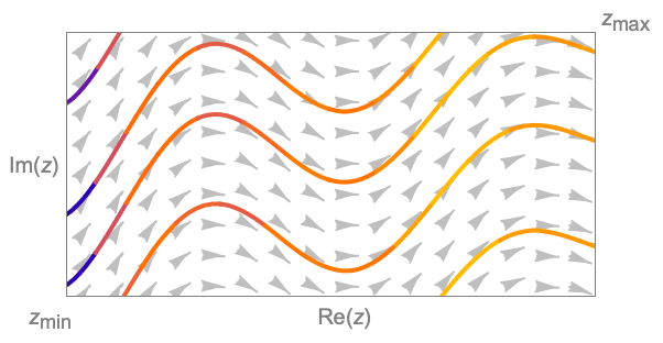
- ComplexStreamPlot 绘制显示每个点处的复向量场的局部方向的流线. 实际上就是求解微分方程

,然后绘制
. - 默认情况下,ComplexStreamPlot 会显示足够多的流线以在整个图中展示大致均匀的密度,并且不显示背景标量场.
- 在对 f 等的值进行计算后,在结果不是复数的位置处不显示流线.
- ComplexStreamPlot[f,{z,n}] 等价于 ComplexStreamPlot[f,{z,-n-n I,n+n I}].
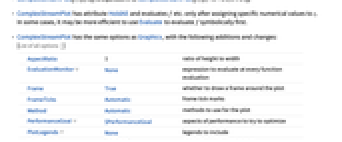
- ComplexStreamPlot 具有属性 HoldAll,只在对 z 赋值后才计算 f 等. 某些情况下,先用 Evaluate 对 f 进行符号式计算效率更高.
- ComplexStreamPlot 和 Graphics 有相同的选项,不同之处和更多选项如下所示: [所有选项的列表]
-
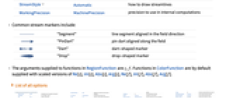
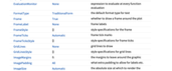
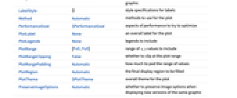
AspectRatio 1 长宽比 EvaluationMonitor None 每次运行函数时要计算的表达式 Frame True 是否为图形绘制边框 FrameTicks Automatic 边框刻度标记 Method Automatic 使用何种方法绘图 PerformanceGoal $PerformanceGoal 优化的目标 PlotLegends None 要包含的图例 PlotRange {Full,Full} 包括的 x、y 值的范围 PlotRangePadding Automatic 对数值范围进行多少填充 PlotTheme $PlotTheme 绘图的整体外观主题 RegionBoundaryStyle Automatic 怎样设置绘图区域边界的样式 RegionFillingStyle Automatic 怎样设置绘图区域内部的样式 RegionFunction (True&) 确定要包含的区域 StreamColorFunction Automatic 如何为流线着色 StreamColorFunctionScaling True 是否缩放传递给 StreamColorFunction 的参数 StreamMarkers Automatic 流的形状 StreamPoints Automatic 确定流线的数量、放置和紧密度 StreamScale Automatic 确定单个流线的大小和分段 StreamStyle Automatic 如何绘制流线 WorkingPrecision MachinePrecision 内部计算使用的精度 - 常见的流线标记有:
-
"Segment" 与场方向一致的线段 

"PinDart" 沿场方向的销镖形 
"Dart" 镖形标记 

"Drop" 水滴形标记 - 提供给 RegionFunction 中的函数的参数为
、
. 默认情况下,为 ColorFunction 中的函数提供的是 Re[z]、Im[z]、Abs[z]、Arg[z]、Re[f]、Im[f]、Abs[f]、Arg[f] 经过缩放的值.
所有选项的列表
范例
打开所有单元 关闭所有单元范围 (22)
采样 (8)
Table[ComplexStreamPlot[z^2, {z, -3 - 3I, 3 + 3I}, PlotLabel -> p, StreamPoints -> p], {p, {Coarse, Medium, Automatic, Fine}}]ComplexStreamPlot[z^2, {z, -3 - 3I, 3 + 3I}, StreamPoints -> {1 + I, 1 - I, 2, -2, 2 + 2I, -2 - 2I}]ComplexStreamPlot[z^2, {z, -3 - 3I, 3 + 3I}, StreamPoints -> {{{1 + I, Red}, {1 - I, Green}, Automatic}}, StreamColorFunction -> None]ComplexStreamPlot[z^2, {z, -3 - 3I, 3 + 3I}, RegionFunction -> Function[{z, f}, Abs[z] < 3]]ComplexStreamPlot[{z^2, Conjugate[z^2]}, {z, -2 - 2I, 2 + 2I}, StreamColorFunction -> None]ComplexStreamPlot[z^2 + 1, {z, -2 - 2I, 2 + 2I}, Mesh -> 5]ComplexStreamPlot[z^2 + 1, {z, -2 - 2I, 2 + 2I}, Mesh -> {{1, 2, 3, 4, 5}}]在赋值前用 Evaluate 符号式计算向量场:
ComplexStreamPlot[Evaluate[D[z^3 + z, z]], {z, -2 - 2I, 2 + 2I}]演示 (14)
通过设置 StreamScale 指定不同的分段长度和箭头:
Table[ComplexStreamPlot[Exp[2z], {z, -2 - 2I, 2 + 2I}, PlotLabel -> ToString@s, StreamScale -> s], {s, {Automatic, None, Full}}]ComplexStreamPlot[Exp[2z], {z, -2 - 2I, 2 + 2I}, StreamColorFunction -> Hue]Table[ComplexStreamPlot[Exp[2z], {z, -2 - 2I, 2 + 2I}, StreamMarkers -> s], {s, {"Toothpick", "Dart", "Drop"}}]ComplexStreamPlot[Exp[2z], {z, -2 - 2I, 2 + 2I}, PlotTheme -> "Business"]ComplexStreamPlot[Exp[2z], {z, -2 - 2I, 2 + 2I}, PlotTheme -> "Business", StreamStyle -> Red, StreamColorFunction -> None]ComplexStreamPlot[Exp[2z], {z, -2 - 2I, 2 + 2I}, StreamColorFunction -> "Rainbow"]ComplexStreamPlot[Exp[2z], {z, -2 - 2I, 2 + 2I}, StreamColorFunction -> None, StreamStyle -> Orange]ComplexStreamPlot[z Exp[2z], {z, -2 - 2I, 2 + 2I}, Mesh -> {{{1, Thick}, {2, Green}, {4, {Thick, Red, Dashed}}}}, MeshStyle -> Opacity[1]]Table[ComplexStreamPlot[z Exp[z], {z, -2 - 2I, 2 + 2I}, Mesh -> 10, MeshStyle -> s], {s, {Red, Thick, Directive[Red, Dashed]}}]ComplexStreamPlot[z Sin[z], {z, -2 - 2I, 2 + 2I}, Mesh -> 10, MeshShading -> {Red, Yellow, Green, None}]regionFn = Function[{z, f}, 4 < Abs[f] < 6 || 0 < Abs[f] < 2];Table[ComplexStreamPlot[z Sin[z], {z, -2 - 2I, 2 + 2I}, RegionFunction -> regionFn, RegionBoundaryStyle -> b], {b, {Red, Thick, Directive[Red, Dashed]}}]ComplexStreamPlot[z Sin[z], {z, -2 - 2I, 2 + 2I}, PlotLegends -> Automatic]ComplexStreamPlot[{z Sin[z], z Cos[z]}, {z, -2 - 2I, 2 + 2I}, PlotLegends -> "Expressions", StreamColorFunction -> None]ComplexStreamPlot[{z Sin[z], z Cos[z]}, {z, -2 - 2I, 2 + 2I}, PlotLegends -> {"first", "second"}, StreamColorFunction -> None]选项 (60)
Background (1)
EvaluationMonitor (2)
PerformanceGoal (2)
PlotLegends (7)
ComplexStreamPlot[Sinc[z], {z, -2 - 2I, 2 + 2I}]ComplexStreamPlot[Sinc[z], {z, -2 - 2I, 2 + 2I}, PlotLegends -> Automatic]ComplexStreamPlot[{Sinc[z], z}, {z, -2 - 2I, 2 + 2I}, PlotLegends -> {"one", "two"}, StreamColorFunction -> None]ComplexStreamPlot[{Sinc[z], z}, {z, -2 - 2I, 2 + 2I}, PlotLegends -> Placed[{"one", "two"}, Below], StreamColorFunction -> None]ComplexStreamPlot[{Sinc[z], z}, {z, -2 - 2I, 2 + 2I}, PlotLegends -> "Expressions", StreamColorFunction -> None]ComplexStreamPlot[{Sinc[z], z}, {z, -2 - 2I, 2 + 2I}, PlotLegends -> Automatic, StreamColorFunction -> None]ComplexStreamPlot[{Sinc[z], z}, {z, -2 - 2I, 2 + 2I}, PlotLegends -> SwatchLegend["Expressions", LegendMarkerSize -> {40, 10}], StreamColorFunction -> None]PlotRange (5)
ComplexStreamPlot[z^3, {z, -2 - 2I, 2 + 2I}, PlotRange -> Full]ComplexStreamPlot[z^3, {z, -2 - 2I, 2 + 2I}, PlotRange -> 1]ComplexStreamPlot[z^3, {z, -2 - 2I, 2 + 2I}, PlotRange -> {{-1, 1}, Automatic}]ComplexStreamPlot[z^3, {z, -2 - 2I, 2 + 2I}, PlotRange -> {Full, {-1, 2}}]ComplexStreamPlot[z^3, {z, -2 - 2I, 2 + 2I}, PlotRange -> {{-2, 1}, {0, 1}}]PlotTheme (3)
ComplexStreamPlot[{Sqrt[z], z^3}, {z, -2 - 2I, 2 + 2I}, PlotTheme -> "Web"]ComplexStreamPlot[{Sqrt[z], z^3}, {z, -2 - 2I, 2 + 2I}, PlotTheme -> "Detailed", StreamColorFunction -> None]ComplexStreamPlot[{Sqrt[z], z^3}, {z, -2 - 2I, 2 + 2I}, PlotTheme -> "Detailed", StreamStyle -> {Red, Blue}, StreamColorFunction -> None]RegionBoundaryStyle (1)
regionFn = Function[{z, f}, n = Norm[z];4 < n < 6 || 0 < n < 2];ComplexStreamPlot[z Sin[z], {z, -2 - 2I, 2 + 2I}, RegionFunction -> regionFn]Table[ComplexStreamPlot[z Sin[z], {z, -2 - 2I, 2 + 2I}, RegionFunction -> regionFn, RegionBoundaryStyle -> b], {b, {Red, Thick, Directive[Red, Dashed]}}]RegionFillingStyle (1)
regionFn = Function[{z, f}, n = Norm[z];4 < n < 6 || 0 < n < 2];ComplexStreamPlot[z Sin[z], {z, -2 - 2I, 2 + 2I}, RegionFunction -> regionFn]ComplexStreamPlot[z Sin[z], {z, -2 - 2I, 2 + 2I}, RegionFunction -> regionFn, RegionFillingStyle -> None]ComplexStreamPlot[z Sin[z], {z, -2 - 2I, 2 + 2I}, RegionFunction -> regionFn, RegionFillingStyle -> Yellow]RegionFunction (3)
ComplexStreamPlot[z^4 + z^2, {z, -2 - 2I, 2 + 2I}, RegionFunction -> Function[{z, f}, Abs[z] < 2]]ComplexStreamPlot[z^4 + z^2, {z, -2 - 2I, 2 + 2I}, RegionFunction -> Function[{z, f}, Abs[f] > 2]]ComplexStreamPlot[z^4 + z^2, {z, -2 - 2I, 2 + 2I}, RegionFunction -> Function[{z, f}, Abs[f] < 1 || Abs[f] > 6]]StreamColorFunction (5)
ComplexStreamPlot[z^4 + z^2, {z, -2 - 2I, 2 + 2I}, StreamColorFunction -> Hue]使用来自 ColorData 的已命名颜色梯度:
ComplexStreamPlot[z^4 + z^2, {z, -2 - 2I, 2 + 2I}, StreamColorFunction -> "Rainbow"]将 ColorData 用于预定义的颜色梯度:
ComplexStreamPlot[z^4 + z^2, {z, -2 - 2I, 2 + 2I}, StreamColorFunction -> Function[{z, f}, ColorData["AvocadoColors"][Arg[z]]]]ComplexStreamPlot[z^4 + z^2, {z, -2 - 2I, 2 + 2I}, StreamColorFunction -> Function[{z, f}, Blend[{Blue, Red}, Re[z]]]]用 StreamColorFunctionScalingFalse 获取未经缩放的值:
ComplexStreamPlot[z^4 + z^2, {z, -2 - 2I, 2 + 2I}, StreamColorFunction -> Hue, StreamColorFunctionScaling -> False]StreamColorFunctionScaling (3)
ComplexStreamPlot[z, {z, -2 - 2I, 2 + 2I}, StreamColorFunction -> Hue]用 StreamColorFunctionScalingFalse 获取未经缩放的值:
ComplexStreamPlot[z, {z, -2 - 2I, 2 + 2I}, StreamColorFunction -> Hue, StreamColorFunctionScaling -> False]ComplexStreamPlot[z, {z, -2 - 2I, 2 + 2I}, StreamColorFunction -> Function[{z, f}, Hue[Abs[f], Abs[z], 1]], StreamColorFunctionScaling -> {True, False}]StreamMarkers (8)
ComplexStreamPlot[z^2 - Conjugate[z], {z, -2 - 2I, 2 + 2I}]ComplexStreamPlot[z^2 - Conjugate[z], {z, -2 - 2I, 2 + 2I}, StreamMarkers -> "Drop"]ComplexStreamPlot[{z, z^2 - Conjugate[z]}, {z, -2 - 2I, 2 + 2I}, StreamMarkers -> {"Drop", "Dart"}, StreamColorFunction -> None]Table[ComplexStreamPlot[z^2 Log[z], {z, -2 - 2I, 2 + 2I}, PlotLabel -> s, StreamStyle -> s], {s, {"Segment", "Line"}}]Table[ComplexStreamPlot[z^2 Log[z], {z, -2 - 2I, 2 + 2I}, PlotLabel -> s, StreamScale -> {Full, All, 0.05}, StreamStyle -> s], {s, {"Arrow", "ArrowArrow", "CircleArrow"}}]Table[ComplexStreamPlot[z^2 Log[z], {z, -2 - 2I, 2 + 2I}, PlotLabel -> s, StreamScale -> {Full, All, 0.03}, StreamStyle -> s], {s, {"BarDot", "Dot", "DotArrow", "DotDot"}}]Table[ComplexStreamPlot[z^2 Log[z], {z, -2 - 2I, 2 + 2I}, PlotLabel -> s, StreamScale -> {Full, All, 0.03}, StreamStyle -> s], {s, {"Drop", "BackwardPointer", "Pointer", "Toothpick"}}]Table[ComplexStreamPlot[z^2 Log[z], {z, -2 - 2I, 2 + 2I}, PlotLabel -> s, StreamScale -> {Full, All, 0.03}, StreamStyle -> s], {s, {"Dart", "PinDart", "DoubleDart"}}]StreamPoints (5)
ComplexStreamPlot[z^2 - Conjugate[z], {z, -2 - 2I, 2 + 2I}, StreamPoints -> 10]Table[ComplexStreamPlot[z^2 - Conjugate[z], {z, -2 - 2I, 2 + 2I}, StreamPoints -> p, PlotLabel -> p], {p, {Automatic, Coarse, Fine}}]ComplexStreamPlot[z^2 - Conjugate[z], {z, -2 - 2I, 2 + 2I}, StreamColorFunction -> None, StreamPoints -> {{{{1, 1}, Red}, {{-1, -1}, Green}, Automatic}}]Table[ComplexStreamPlot[z^2 - Conjugate[z], {z, -2 - 2I, 2 + 2I}, StreamPoints -> {Automatic, d}], {d, {Automatic, 1, Scaled[0.05]}}]Table[ComplexStreamPlot[z^2 - Conjugate[z], {z, -2 - 2I, 2 + 2I}, StreamPoints -> {Automatic, d}], {d, {Automatic, {Scaled[0.1], Scaled[0.5]}}}]StreamScale (9)
ComplexStreamPlot[z^3 - Conjugate[z], {z, -2 - 2I, 2 + 2I}, StreamScale -> Full]ComplexStreamPlot[z^3 - Conjugate[z], {z, -2 - 2I, 2 + 2I}, StreamScale -> None]Table[ComplexStreamPlot[z^3 - Conjugate[z], {z, -2 - 2I, 2 + 2I}, PlotLabel -> s, StreamScale -> s], {s, {Tiny, Large}}]Table[ComplexStreamPlot[z^3 - Conjugate[z], {z, -2 - 2I, 2 + 2I}, PlotLabel -> s, StreamScale -> s], {s, {0.1, 0.2, 0.4}}]ComplexStreamPlot[z^3 - Conjugate[z], {z, -2 - 2I, 2 + 2I}, StreamScale -> {{0.1, 0.1}, Automatic}]Table[ComplexStreamPlot[z^3 - Conjugate[z], {z, -2 - 2I, 2 + 2I}, PlotLabel -> n, StreamScale -> {Full, n}], {n, {12, 24, All}}]Table[ComplexStreamPlot[z^3 - Conjugate[z], {z, -2 - 2I, 2 + 2I}, PlotLabel -> a, StreamScale -> {Automatic, Automatic, a}], {a, {.02, .04}}]Table[ComplexStreamPlot[z^3 - Conjugate[z], {z, -2 - 2I, 2 + 2I}, PlotLabel -> a, StreamScale -> {Automatic, Automatic, a}], {a, {Scaled[0.5], Scaled[1], Scaled[1.5]}}]ComplexStreamPlot[z^3 - Conjugate[z], {z, -2 - 2I, 2 + 2I}, StreamScale -> {Automatic, 2, Automatic, Function[{z, f}, Re[z]]}]StreamStyle (5)
对于颜色,StreamColorFunction 比 StreamStyle 的优先级高:
ComplexStreamPlot[z^2 Log[z], {z, -2 - 2I, 2 + 2I}, StreamStyle -> Red]设置 StreamColorFunctionNone,用 StreamStyle 指定颜色:
ComplexStreamPlot[z^2 Log[z], {z, -2 - 2I, 2 + 2I}, StreamStyle -> Red, StreamColorFunction -> None]Table[ComplexStreamPlot[z^2 Log[z], {z, -2 - 2I, 2 + 2I}, StreamStyle -> s, StreamColorFunction -> None], {s, {Orange, Thick, Directive[Orange, Dashed]}}]ComplexStreamPlot[z^2 Log[z], {z, -2 - 2I, 2 + 2I}, StreamScale -> Full, StreamStyle -> Arrowheads[{{0.03, Automatic, Graphics[Circle[]]}}]]ComplexStreamPlot[{z, z^2 Log[z]}, {z, -2 - 2I, 2 + 2I}, StreamStyle -> {Red, Blue}, StreamColorFunction -> None]应用 (10)
基本应用 (1)
ComplexStreamPlot[z, {z, 5}]ComplexStreamPlot[z + 1, {z, 5}]ComplexStreamPlot[z ^ 2, {z, 5}]ComplexStreamPlot[Sqrt[z], {z, 5}]ComplexStreamPlot[Sin[z], {z, 5}]ComplexStreamPlot[Log[z], {z, 5}]ComplexStreamPlot[1 / z, {z, 5}]ComplexStreamPlot[1 / z ^ 2, {z, 5}]其他应用 (9)
ComplexStreamPlot[z, {z, -3 - 3I, 3 + 3I}]ComplexStreamPlot[-z, {z, -3 - 3I, 3 + 3I}]
,与复变函数
对应的实向量场为
,场的轨迹满足微分方程
. 隐式解为
,
为实数,对应于在原点与实轴相切的一组圆:
Show[ContourPlot[(x^2/y) + y, {x, -3, 3}, {y, -3, 3}, ContourShading -> None, ContourStyle -> Red, Contours -> Range[-8, 8]], ComplexStreamPlot[z^2, {z, -3 - 3I, 3 + 3I}, StreamColorFunction -> None]]Show[PolarPlot[Evaluate@Table[c Sin[θ], {c, -3, 3}], {θ, 0, π}, PlotStyle -> Red], ComplexStreamPlot[z^2, {z, -3 - 3I, 3 + 3I}, StreamColorFunction -> None]]n = 4;Show[PolarPlot[Evaluate@Table[c Surd[Sin[(n - 1)θ], n - 1], {c, -3, 3}], {θ, 0, π}, PlotStyle -> Red], ComplexStreamPlot[z^n, {z, -3 - 3I, 3 + 3I}, StreamColorFunction -> None]]n = -4;Show[PolarPlot[Evaluate@Table[c Surd[Sin[(n - 1)θ], n - 1], {c, -3, 3}], {θ, 0, π}, PlotStyle -> Red], ComplexStreamPlot[z^n, {z, -3 - 3I, 3 + 3I}, StreamColorFunction -> None], PlotRange -> 3]在阶数
的零点附近,流线形成了几个圈,在
个方向上起于零点,终于零点:
n = 3;Show[ComplexPlot[z^n, {z, -3 - 3I, 3 + 3I}, ColorFunction -> None], ComplexStreamPlot[z^n, {z, -3 - 3I, 3 + 3I}, StreamStyle -> White, StreamColorFunction -> None, StreamScale -> Large]]在
阶极点附近,流线从
个方向汇聚到极点,然后从极点出发向
个方向发散:
n = 2;Show[ComplexPlot[1 / z^n, {z, -3 - 3I, 3 + 3I}, ColorFunction -> None], ComplexStreamPlot[1 / z^n, {z, -3 - 3I, 3 + 3I}, StreamStyle -> White, StreamColorFunction -> None, StreamScale -> Large]]函数
在
和
处有简单零点,在
处有 1 阶极点,在
处有一个 2 阶极点:
ComplexStreamPlot[(z^2 + 2 z - 3/z^4 - 6 z^3 + 18 z^2 - 54 z + 81), {z, -5 - 5I, 5 + 5I}]ComplexStreamPlot[Exp[-5 / z], {z, -1 - I, 1 + I}]ComplexStreamPlot[#, {z, -1 - I, 1 + I}]& /@ NestList[D[#, z]&, z^3, 3]ComplexStreamPlot[Conjugate[z^2], {z, -2 - 2I, 2 + 2I}]令
为理想流体的复势.
为速度势,
为流函数,流体的速度场为
. 根据 Cauchy–Riemann 方程,
,因此可以用
的共轭来生成流线图. 显示流体流过圆柱时的循环流线图:
F = z + (1/z) + I Log[z];ComplexStreamPlot[Evaluate[Conjugate[D[F, z]]], {z, -2 - 2I, 2 + 2I}, Epilog -> {Circle[]}, StreamScale -> Full, StreamStyle -> "Line"]F = (-I z)^2 / 3 - (-z)^2 / 3;ComplexStreamPlot[Evaluate[Conjugate[D[F, z]]], {z, -2 - 2I, 2 + 2I}, StreamScale -> Full, StreamStyle -> "Line", RegionFunction -> Function[{z, f}, Arg[z] < -π / 2 || Arg[z] > 0]]属性和关系 (15)
ComplexStreamPlot 是 StreamPlot 的特例:
{ComplexStreamPlot[Sin[z], {z, 4}], StreamPlot[ReIm[Sin[x + I * y]], {x, -4 , 4}, {y, -4, 4}]}ComplexVectorPlot 将复数绘制为向量:
ComplexVectorPlot[Log[z], {z, 3}]ComplexVectorPlot 是 VectorPlot 的特殊情况:
VectorPlot[ReIm[Log[x + I y]], {x, -3, 3}, {y, -3, 3}]使用 VectorDisplacementPlot 可视化指定区域内的复函数效果:
VectorDisplacementPlot[ReIm[Sin[x + I y]], {x, y}∈Annulus[], VectorPoints -> Automatic, VectorSizes -> Full]用 VectorPlot3D 和 StreamPlot3D 可视化三维向量场:
{VectorPlot3D[{z, x, y}, {x, -1, 1}, {y, -1, 1}, {z, -1, 1}], StreamPlot3D[{z, x, y}, {x, -1, 1}, {y, -1, 1}, {z, -1, 1}]}ComplexContourPlot 绘制复平面上的曲线:
ComplexContourPlot[Abs[Log[z]] == 1, {z, 3}]ComplexRegionPlot 绘制复平面上的区域:
ComplexRegionPlot[Abs[Log[z]] < 1, {z, 3}]ComplexPlot 用颜色显示函数的辐角和幅值:
ComplexPlot[Log[z], {z, 3}]通过 ComplexPlot3D 用
轴显示幅值:
ComplexPlot3D[Log[z], {z, 3}]用 ComplexArrayPlot 绘制复数数组:
ComplexArrayPlot[Table[x ^ 3 + I y ^ 2, {x, -2, 2, 0.1}, {y, -2, 2, 0.1}]]用 ReImPlot 和 AbsArgPlot 在实平面上绘制复数:
ReImPlot[Log[x], {x, -3, 3}]AbsArgPlot[Log[x], {x, -3, 3}]用 ComplexListPlot 显示复数在平面上的位置:
ComplexListPlot[RandomComplex[{-3 - 3I, 3 + 3I}, 100]]使用 ListVectorPlot 绘制数据:
data = Table[ReIm[(x + I y)^2], {x, -3, 3, 0.2}, {y, -3, 3, 0.2}];ListVectorPlot[data]使用 ListStreamPlot 绘制流线图而非向量:
ListStreamPlot[data]使用 VectorDensityPlot 添加标量场的密度图:
VectorDensityPlot[ReIm[(x + I y)^2], {x, -3, 3}, {y, -3, 3}]StreamDensityPlot 可使用流线图而非向量:
StreamDensityPlot[ReIm[(x + I y)^2], {x, -3, 3}, {y, -3, 3}]使用 ListVectorDensityPlot 生成基于数据的标量场的密度图:
data = Table[{{x, y}, ReIm[(x + I y)^2 + 1]}, {x, -3, 3, 0.2}, {y, -3, 3, 0.2}];ListVectorDensityPlot[data]使用 ListStreamDensityPlot 绘制流线图而非向量:
ListStreamDensityPlot[data]使用 LineIntegralConvolutionPlot 绘制向量场的线积分卷积:
LineIntegralConvolutionPlot[ReIm[(x + I y)^3], {x, -3, 3}, {y, -3, 3}]文本
Wolfram Research (2020),ComplexStreamPlot,Wolfram 语言函数,https://reference.wolfram.com/language/ref/ComplexStreamPlot.html (更新于 2020 年).
CMS
Wolfram 语言. 2020. "ComplexStreamPlot." Wolfram 语言与系统参考资料中心. Wolfram Research. 最新版本 2020. https://reference.wolfram.com/language/ref/ComplexStreamPlot.html.
APA
Wolfram 语言. (2020). ComplexStreamPlot. Wolfram 语言与系统参考资料中心. 追溯自 https://reference.wolfram.com/language/ref/ComplexStreamPlot.html 年
BibTeX
@misc{reference.wolfram_2026_complexstreamplot, author="Wolfram Research", title="{ComplexStreamPlot}", year="2020", howpublished="\url{https://reference.wolfram.com/language/ref/ComplexStreamPlot.html}", note=[Accessed: 08-September-2026]}
BibLaTeX
@online{reference.wolfram_2026_complexstreamplot, organization={Wolfram Research}, title={ComplexStreamPlot}, year={2020}, url={https://reference.wolfram.com/language/ref/ComplexStreamPlot.html}, note=[Accessed: 08-September-2026]}