ExponentialPowerDistribution

ExponentialPowerDistribution[κ,μ,σ]

形状母数 κ，位置母数 μ，尺度母数 σ の指数ベキ分布を表す．

ExponentialPowerDistribution[κ]

位置母数0，尺度母数1の指数ベキ分布を表す．

詳細

ExponentialPowerDistributionは一般化された正規分布としても知られている．
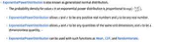
指数ベキ分布における値の確率密度は $exp(-(TemplateBox[{{x, -, mu}}, Abs]^kappa)/(kappa sigma^kappa))$ に比例する．
ExponentialPowerDistributionでは，κ と σ は任意の正の実数で，μ は任意の実数でよい．
ExponentialPowerDistributionでは，μ と σ は単位次元が等しい任意の数量でよく，κ は無次元量でよい． »
ExponentialPowerDistributionは，Mean，CDF，RandomVariate等の関数とともに使うことができる．

予備知識

ExponentialPowerDistribution[κ,μ,σ]は，実数集合上で定義され，実数 μ （「位置母数」と呼ばれる）と2つの正の実数 κ および σ（それぞれ「形状母数」および「尺度母数」と呼ばれる）でパラメータ化された連続統計分布を表す．母数 μ は，指数ベキ分布の確率密度関数(PDF)の「峰」（つまり，絶対最大値）の水平位置を決定する．PDFは常に単峰であるが，グラフの全体的な高さや傾きは κ および σ の値によって決定される．加えて，PDFの裾部はの大きい値についてPDFが指数的にではなく代数的に減少するという意味で「厚い」（この動作は分布のSurvivalFunctionを分析することで数量的に正確にできる）．指数ベキ分布は一般化した正規分布と呼ばれることがあるが，この言葉は非対称分布の無関係な族を指すことがあるので注意が必要である．
指数ベキ分布は，形状母数 κ を加える一般化された正規分布(NormalDistribution) と考えることができる．この変化形は，対称ではあるが「広がり」が大きく，高さは高く，「点が鋭い」（つまり，微分が不可能な点）分布になる．指数ベキ分布は，1970年代の中頃，Robert SmithおよびLee Bainによって，寿命モデルとして初めて提案された．この分布は，それ以来，さまざまな種類のガンに罹患している患者の生存率，運動選手の血漿集中測定，製造業で使用される物質が割れる頻度，金融市場で支払われる利益等の，数多くの現象のモデル化に使われている．
RandomVariateを使って指数ベキ分布から，1つあるいは複数の機械精度あるいは任意精度（後者はWorkingPrecisionオプションを介す）の擬似乱数変量を得ることができる．Distributed[x,ExponentialPowerDistribution[κ,μ,σ]]（より簡略すると xExponentialPowerDistribution[κ,μ,σ]）を使って，確率変数 x が，指数ベキ分布に従って分布していると宣言することができる．このような宣言は，Probability，NProbability，Expectation，NExpectation等の関数で使うことができる．
確率密度関数および累積分布関数は，PDF[ExponentialPowerDistribution[κ,μ,σ],x]およびCDF[ExponentialPowerDistribution[κ,μ,σ],x]を使って得られることがある．平均，中央値，分散，原点の周りのモーメント，中心モーメントは，それぞれMean，Median，Variance，Moment，CentralMomentを使って計算することができる．
DistributionFitTestを使って，与えられたデータ集合が指数ベキ分布と一致するかどうかを検定することが，EstimatedDistributionを使って与えられたデータからパラメトリック指数ベキ分布を推定することが，FindDistributionParametersを使ってデータを指数ベキ分布にフィットすることができる．ProbabilityPlotを使って記号指数ベキ分布のCDFに対する与えられたデータのCDFのプロットを生成することが，QuantilePlotを使って記号指数ベキ分布の変位値に対する与えられたデータの変位値のプロットを生成することができる．
TransformedDistributionを使って変換された指数ベキ分布を表すことが，CensoredDistributionを使って上限値と下限値の間で切り取られた値の分布を表すことが，TruncatedDistributionを使って上限値と下限値の間で切断された値の分布を表すことができる．CopulaDistributionを使って指数ベキ分布を含む高次元分布を構築することが，ProductDistributionを使って指数ベキ分布を含む独立成分分布の結合分布を計算することができる．
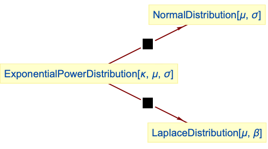
指数ベキ分布は他の多くの分布に関連している．例えば，ExponentialPowerDistribution[2,μ,σ]のPDFがNormalDistribution[μ,σ]のそれと同じであるという意味で，ExponentialPowerDistributionは，NormalDistributionの明らかな一般化である．ExponentialPowerDistributionは，ExponentialPowerDistribution[1,μ,β]がLaplaceDistribution[μ,β]と同じCDFを持つという意味で，LaplaceDistributionの一般化でもある．DirichletDistributionからの確率ベクトルの長さの分布はExponentialPowerDistributionによって平滑にモデル化することができる．加えて，ExponentialPowerDistributionはStudentTDistribution，ChiDistribution，MaxwellDistribution，RayleighDistribution，RiceDistributionと定性的に関係している．

例題

すべて開くすべて閉じる

例 (4)

確率密度関数：

Wolfram Language code:

Plot[Table[PDF[ExponentialPowerDistribution[κ, 1, 3], x], {κ, {1 / 2, 1.5, 6}}]//Evaluate, {x, -5, 8}, Filling -> Axis, Exclusions -> None]

Wolfram Language code:

Plot[Table[PDF[ExponentialPowerDistribution[3, μ, .8], x], {μ, {-1 / 2, 1, 2}}]//Evaluate, {x, -3, 5}, Filling -> Axis, Exclusions -> None]

Wolfram Language code:

Plot[Table[PDF[ExponentialPowerDistribution[3, 1, σ], x], {σ, {0.7, 1.1, 2}}]//Evaluate, {x, -3, 5}, Filling -> Axis, Exclusions -> None]

Wolfram Language code: PDF[ExponentialPowerDistribution[κ, μ, σ], x]

累積分布関数：

Wolfram Language code:

Plot[Table[CDF[ExponentialPowerDistribution[κ, 1, 3], x], {κ, {1 / 2, 1.5, 6}}]//Evaluate, {x, -5, 8}, Filling -> Axis, Exclusions -> None]

Wolfram Language code:

Plot[Table[CDF[ExponentialPowerDistribution[3, μ, .8], x], {μ, {-1 / 2, 1, 2}}]//Evaluate, {x, -3, 5}, Filling -> Axis, Exclusions -> None]

Wolfram Language code:

Plot[Table[CDF[ExponentialPowerDistribution[3, 1, σ], x], {σ, {0.7, 1.1, 2}}]//Evaluate, {x, -3, 5}, Filling -> Axis, Exclusions -> None]

Wolfram Language code: CDF[ExponentialPowerDistribution[κ, μ, σ], x]

平均と分散：

Wolfram Language code: Mean[ExponentialPowerDistribution[κ, μ, σ]]

Wolfram Language code: Variance[ExponentialPowerDistribution[κ, μ, σ]]

中央値：

Wolfram Language code: Median[ExponentialPowerDistribution[κ, μ, σ]]

スコープ (8)

指数ベキ分布から擬似乱数のサンプルを生成する：

Wolfram Language code: data = RandomVariate[ExponentialPowerDistribution[3, 1, 2], 10 ^ 4];

そのヒストグラムを確率密度関数と比較する：

Wolfram Language code:

Show[
	Histogram[data, 20, "PDF"], 
	Plot[PDF[ExponentialPowerDistribution[3, 1, 2], x], {x, Min[data], Max[data]}, PlotStyle -> Thick]]

分布母数推定：

Wolfram Language code: sample = RandomVariate[ExponentialPowerDistribution[2, 1, 3], 10 ^ 3];

サンプルデータから分布母数を推定する：

Wolfram Language code: edist = EstimatedDistribution[sample, ExponentialPowerDistribution[k, μ, σ]]

サンプルの密度ヒストグラムを推定分布の確率密度関数と比較する：

Wolfram Language code: Show[Histogram[sample, Automatic, "PDF"], Plot[PDF[edist, x], {x, Min[sample], Max[sample]}, PlotStyle -> Thick]]

指数ベキ分布は対称性を有する：

Wolfram Language code: Skewness[ExponentialPowerDistribution[κ, μ, σ]]

尖度は形状母数 κ のみに依存する：

Wolfram Language code: Plot[Kurtosis[ExponentialPowerDistribution[κ, μ, σ]], {κ, 0, 10}, Filling -> Axis]

Wolfram Language code: Kurtosis[ExponentialPowerDistribution[κ, μ, σ]]

尖度の極限値：

Wolfram Language code: Limit[Kurtosis[ExponentialPowerDistribution[κ, μ, σ]], κ -> ∞]

母数の関数としての閉じた形の種々のモーメント：

Wolfram Language code: FormulaGrid[list_, type_] := Grid[...]

Moment：

Wolfram Language code: FormulaGrid[Table[Moment[ExponentialPowerDistribution[κ, μ, σ], k], {k, 5}], M]

CentralMoment：

Wolfram Language code: FormulaGrid[Table[CentralMoment[ExponentialPowerDistribution[κ, μ, σ], k], {k, 5}], CM]

FactorialMoment：

Wolfram Language code: FormulaGrid[Table[FactorialMoment[ExponentialPowerDistribution[κ, μ, σ], k]//Simplify, {k, 5}], FM]

Cumulant：

Wolfram Language code: FormulaGrid[Table[Cumulant[ExponentialPowerDistribution[κ, μ, σ], k], {k, 5}], C]

ハザード関数は形状母数 κ によって形が異なる：

Wolfram Language code:

Plot[Table[HazardFunction[ExponentialPowerDistribution[κ, 3, 2], x], {κ, {1 / 2, 2, 6}}]//Evaluate, {x, -5, 5}, Filling -> Axis, Exclusions -> None]

分位関数：

Wolfram Language code:

Plot[Table[Quantile[ExponentialPowerDistribution[κ, 3, .2], q], {κ, {0.5, 1, 3}}]//Evaluate, {q, 0, 1}, Exclusions -> None, Filling -> Axis]

Wolfram Language code: Quantile[ExponentialPowerDistribution[κ, μ, σ], q]

母数でQuantityを一貫して使うとQuantityDistributionが与えられる：

Wolfram Language code: len𝒟 = ExponentialPowerDistribution[Quantity[3, "Percent"], Quantity[5.2, "Yards"], Quantity[10, "Yards"]]

QuartileDeviationを求める：

Wolfram Language code: QuartileDeviation[len𝒟]

アプリケーション (1)

ExponentialPowerDistributionはDirichletDistributionに従う確率ベクトルの長さの分布の平滑化近似として使うことができる：

Wolfram Language code: len𝒟 = TransformedDistribution[Sqrt[u ^ 2 + v ^ 2], {u, v}DirichletDistribution[{3, 2, 1}]];

確率密度関数：

Wolfram Language code: pdf = PDF[len𝒟, x]

サンプルを作る：

Wolfram Language code: lens = RandomVariate[len𝒟, 10 ^ 4];

指数ベキ分布をデータにフィットする：

Wolfram Language code:

edist = EstimatedDistribution[lens, ExponentialPowerDistribution[κ, μ, σ], ParameterEstimator -> {"MaximumLikelihood", MaxIterations -> 500}]

サンプルのヒストグラムを両分布の確率密度関数と比較する：

Wolfram Language code:

Show[Histogram[lens, 20, "PDF"], Plot[{PDF[edist, x], pdf}, {x, 0, 1}, PlotRange -> All, PlotStyle -> Thick, PlotLegends -> {"exponential power", "length of Dirichlet vector"}]]

平均を比べる：

Wolfram Language code: {Mean[len𝒟], Mean[edist]}

Wolfram Language code: N[%]

特性と関係 (5)

指数ベキ分布は平行移動と正の因子によるスケーリングの下では閉じている：

Wolfram Language code: TransformedDistribution[a * u + loc, uExponentialPowerDistribution[κ]]

任意の平均とスケールパラメータで：

Wolfram Language code: TransformedDistribution[a * u + loc, uExponentialPowerDistribution[κ, μ, σ]]

ExponentialPowerDistributionは形状母数 κ の値によってNormalDistributionよりも狭くも広くもなる：

Wolfram Language code:

{mean, sd} = {Mean[ExponentialPowerDistribution[κ, μ, σ]], StandardDeviation[ExponentialPowerDistribution[κ, μ, σ]]}

Wolfram Language code:

Block[{μ = 0, σ = 4}, Table[Plot[{PDF[NormalDistribution[mean, sd], x], PDF[ExponentialPowerDistribution[κ, μ, σ], x]}, {x, -10, 10}, PlotRange -> All, PlotLabel -> Row[{"κ =", Text[κ]}]], {κ, {1.3, 1.7, 2.5, 4}}]]

他の分布との関係：

LaplaceDistributionは指数ベキ分布の特殊ケースである：

Wolfram Language code: CDF[ExponentialPowerDistribution[1, μ, β], x]

Wolfram Language code: CDF[LaplaceDistribution[μ, β], x]

Wolfram Language code: % - %%//FullSimplify

NormalDistributionはExponentialPowerDistributionの特殊ケースである：

Wolfram Language code: PDF[ExponentialPowerDistribution[2, μ, σ], x]

Wolfram Language code: PDF[NormalDistribution[μ, σ], x]

Wolfram Language code: % - %%//FullSimplify

おもしろい例題 (1)

累積分布関数の等高線を持つ κ のさまざまな値についての確率密度関数：

Wolfram Language code:

dist = ExponentialPowerDistribution[κ];cdf = Function[{x, κ}, Evaluate[CDF[dist, x]]];
ql = {0.025, 0.10, 0.25, 0.5, 0.75, 0.90, 0.975};
cl = Table[ColorData["Rainbow"][q], {q, Join[{0.0}, ql]}];

Wolfram Language code:

Legended[Plot3D[PDF[dist, x], {x, -3, 3}, {κ, 0.2, 4}, PlotTheme -> "Marketing", MeshFunctions -> {cdf}, Mesh -> {ql}, MeshStyle -> GrayLevel[0.8], MeshShading -> cl, AxesLabel -> Automatic, BaseStyle -> Opacity[0.9], ImageSize -> 400, PlotRange -> All], BarLegend["Rainbow", ql, LegendLabel -> "prob"]]

Top

その他のラーニングリソース

テクニカルサポート

データサイエンス，金融，ビジネス

工学

科学とテクノロジー

教育のためのテクノロジー

教育イニシアチブ

使い始める

Grow Your Skills

Wolframと繋がる

大人用の教育プログラム

若者のための教育プログラム

読む

ExponentialPowerDistribution

詳細

予備知識

例題

例 (4)

スコープ (8)

アプリケーション (1)

特性と関係 (5)

おもしろい例題 (1)

テキスト

CMS

APA

BibTeX

BibLaTeX

ExponentialPowerDistribution

詳細

予備知識

例題

例 (4)

スコープ (8)

アプリケーション (1)

特性と関係 (5)

おもしろい例題 (1)

関連項目

関連するガイド

履歴

テキスト

CMS

APA

BibTeX

BibLaTeX