FiniteField[p,d]
gives a finite field with ![]() elements.
elements.
FiniteField[p,f]
gives the finite field ![]() , where
, where ![]() is an irreducible polynomial in
is an irreducible polynomial in ![]() .
.


FiniteField
FiniteField[p,d]
gives a finite field with ![]() elements.
elements.
FiniteField[p,f]
gives the finite field ![]() , where
, where ![]() is an irreducible polynomial in
is an irreducible polynomial in ![]() .
.
FiniteField[p,…,rep]
uses field element representation rep, either "Polynomial" or "Exponential".
Details
- Finite fields are also known as Galois fields.
- Finite fields are used in algebraic computation, error-correcting codes, cryptography, combinatorics, algebraic geometry, number theory and finite geometry.
- A field
 is an algebraic system with all four arithmetic operations +, -, * and ÷. A finite field
  can have
  elements
  for some prime
  and positive integer
  .
. - The
 element
  is the additive identity where
  for all
  and the
  element
  gives the multiplicative identity where
  for all
  .
. - FiniteFieldElement[,k] or [k] can be used to get the
 element
  and is formatted as
  .
.
- FiniteFieldElement objects in the same field are automatically combined by arithmetic operations.
- Polynomial operations such as PolynomialGCD, Factor, Expand, PolynomialQuotientRemainder and Resultant can be used for polynomials with coefficients from a finite field. Together and Cancel can be used for rational functions with coefficients from a finite field.
- Linear algebra operations such as Det, Inverse, RowReduce, NullSpace, MatrixRank and LinearSolve can be used for matrices with entries from a finite field.
- Solve and Reduce can be used to solve systems of equations over finite fields.
- There are two different representations rep supported for FiniteField: "Polynomial" and "Exponential".
- The "Polynomial" representation is the analog of a Cartesian representation of complex numbers
 , easy to add and subtract but slightly harder to multiply and divide.
 - Representation: It uses an irreducible polynomial
 of degree d to identify the field with the quotient:
  .
. - Each element
 is represented as a polynomial
  . Or you can think of it as a vector
  in the basis
  .
. - Enumeration: The elements are enumerated in reverse lexicographic order:
 ,
, ,…,
,…, ,…,
,…,
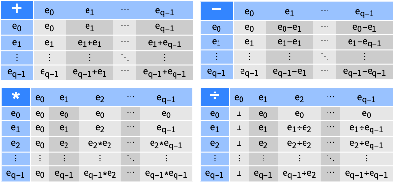
- Operations: Let
 and
and  ; then you have:
  and
and 
- and
 is reduced modulo
  (PolynomialRemainder) to degree
  .
.  with
with  .
.  , and the multiplicative inverse
  is computed using the extended polynomial GCD. Since
  is irreducible, you have
  and hence from the extended polynomial GCD, you have
  for some polynomials
  and
and  . By reducing modulo
  , you get
  and hence you have
  .
. - The "Exponential" representation is the analog of a polar representation of complex number
 , easy to multiply and divide but slightly harder to add and subtract.
 - Representation: As in the "Polynomial" representation, it uses an irreducible polynomial
 of degree d, but in this case
  also needs to be primitive. Since
  is primitive, the powers of
  represent every element in
  except
  :
: -

- This representation is also known as the cyclic group representation, since
 is a cyclic group under multiplication.
 - Enumeration: The elements are enumerated using the power order:
 ,
,  ,
,  , …,
, …,  , …,
, …, 
- Operations: Let
 and
and  , then you have:
 ![u *v=alpha^(TemplateBox[{{(, {i, +, j}, )}, {(, {q, -, 1}, )}}, Mod])](Files/FiniteField.en/73.png "u *v=alpha^(TemplateBox[{{(, {i, +, j}, )}, {(, {q, -, 1}, )}}, Mod])") and
and 
- with the inversion
 . For addition and subtraction, there is no simple rule that gives
  such that
  , and so that is stored in a lookup table that is linear in the field size
  . This makes the operation fast at the cost of storing data. It also means that the "Exponential" representation is not suitable for large fields.
 - The practical difference between representations is:
- "Polynomial" takes no time to create, uses no extra memory, works for large fields but has slightly slower operations.
- "Exponential" takes some time to create, uses extra memory proportional to the size of the field, works for small fields but has slightly faster operations.
- Information[FiniteField[…], prop] gives the property prop of the finite field. The following properties can be specified:
-
"Characteristic" the characteristic p of the finite field "ExtensionDegree" the extension degree d of the finite field over 
"FieldSize" the number of elements q=pd of the field "FieldIrreducible" the polynomial function f used to construct the field "ElementRepresentation" "Polynomial" or "Exponential"
Examples
open all close allBasic Examples (2)
ℱ = FiniteField[5, 1]{ℱ[3] + ℱ[4], ℱ[2] ℱ[4]}Factor[2x ^ 2 + 3x + 1, Extension -> ℱ]Represent a finite field with characteristic ![]() and extension degree
and extension degree ![]() :
:
ℱ = FiniteField[17, 3]Specify elements of the field using polynomial coefficients or an index:
{a, b} = {ℱ[{1, 2, 3}], ℱ[123]}(a ^ 2 + 2b) / (5a b - 7)PolynomialRemainder[x ^ 5 - 1, a x ^ 3 + b x + a b, x]Scope (16)
Representation and Properties (4)
Represent a finite field with characteristic ![]() and extension degree
and extension degree ![]() :
:
ℱ = FiniteField[1009, 3]Find the irreducible polynomial used to construct the field:
Information[ℱ, "FieldIrreducible"]By default, the polynomial representation of field elements is used:
Information[ℱ, "ElementRepresentation"]Find other properties of the field:
Information[ℱ, {"Characteristic", "ExtensionDegree", "FieldSize"}]Field additive and multiplicative identity elements have indices ![]() and
and ![]() :
:
ℱ[123] - ℱ[123]ℱ[345] / ℱ[345]Construct a finite field using a custom irreducible polynomial:
f = 2# ^ 4 + 57# ^ 3 + 43 # ^ 2 + 17# - 500&;Verify that the polynomial is irreducible:
IrreduciblePolynomialQ[f[x], Modulus -> 509]ℱ = FiniteField[509, f, "Polynomial"]The field irreducible is equal to the specified polynomial modulo the field characteristic:
PolynomialMod[Information[ℱ, "FieldIrreducible"][x] - f[x], 509]Construct a finite field that uses exponential representation of elements:
ℱ = FiniteField[7, 3, "Exponential"]The polynomial used to represent the field is primitive:
PrimitivePolynomialQ[Information[ℱ, "FieldIrreducible"][x], 7]Field additive and multiplicative identity elements have indices ![]() and
and ![]() :
:
ℱ[21] - ℱ[21]ℱ[32] / ℱ[32]All nonzero elements of the field are powers of the element with index ![]() :
:
q = Information[ℱ, "FieldSize"]θ = ℱ[2]And@@Table[ℱ[ind] == θ ^ (ind - 1), {ind, q - 1}]FiniteField[11]% === FiniteField[11, 1]Represent a finite field with 49 elements:
FiniteField[49]% === FiniteField[7, 2]Arithmetic (3)
Perform arithmetic operations in a finite field:
ℱ = FiniteField[3, 6];
{a, b} = {ℱ[123], ℱ[432]}{a + b, a - b, a b, a / b, a ^ 321}Rational powers work only with exponent denominators ![]() and
and ![]() :
:
{a ^ (1 / 3), Sqrt[a]}For some field elements, the square root may not exist:
Sqrt[b]Arithmetic operations treat integers as elements of the field:
ℱ = FiniteField[19, 3];
a = ℱ[123]{a + 5, 7a}Rational numbers need to be valid modulo the field characteristic:
a + 7 / 8a + 2 / 19Use Element to decide which rational numbers can be identified with field elements:
{Element[7 / 8, ℱ], Element[2 / 19, ℱ]}For the purpose of comparison, rational numbers are identified with field elements:
ℱ[0] == 0ℱ[1] == 1Elements of different finite fields cannot be combined:
ℱ = FiniteField[389, 2];
𝒢 = FiniteField[389, 4];ℱ[123] - 𝒢[123]Fields with same characteristic and field irreducible but different element representations are allowed:
ℋ = FiniteField[389, Information[ℱ, "FieldIrreducible"], "Exponential"];ℱ[123] - ℋ[123]Automorphisms and Embeddings (2)
Compute all conjugates of a finite field element:
ℱ = FiniteField[7, 5];
a = ℱ[123]conj = Table[FrobeniusAutomorphism[a, i], {i, 0, 4}]The conjugates are roots of the minimal polynomial of a:
f = MinimalPolynomial[a]f /@ conjThe Frobenius automorphism maps ![]() to
to ![]() :
:
FrobeniusAutomorphism[a] == a ^ 7Compute an embedding of one finite field in another:
𝒦 = FiniteField[29, 3];
ℱ = FiniteField[29, 6];
emb = FiniteFieldEmbedding[𝒦, ℱ]
Map finite field elements through the embedding:
emb[𝒦[123]]Embeddings preserve arithmetic operations:
{a, b} = {𝒦[345], 𝒦[678]};emb[a + b] == emb[a] + emb[b]emb[a b] == emb[a]emb[b]Polynomials over Finite Fields (2)
Compute with polynomials over a finite field:
ℱ = FiniteField[11, 3];
f = ℱ[1]x ^ 2 + ℱ[2]x + ℱ[3];
g = ℱ[12]x ^ 5 + ℱ[21]x + ℱ[33];
h = ℱ[321]x ^ 3 + ℱ[27]x ^ 2 + ℱ[53]x + ℱ[19];fg = Expand[f g]gh = Expand[g h]gcd = PolynomialGCD[fg, gh]Cancel[gcd / g]Compute quotient and remainder:
{q, r} = PolynomialQuotientRemainder[g, h, x]Expand[g - q h - r]Factor[h]Resultant[f, g, x]Compute with multivariate polynomials:
Expand[(f y + g z)(h z + 1)]Factor[%]Discriminant[f y ^ 2 + g y + h, y]Factor a polynomial over an extension of a finite field:
ℱ = FiniteField[29, 3];
f = ℱ[12]x ^ 2 + ℱ[34]x + ℱ[56];
The polynomial ![]() is irreducible over
is irreducible over ![]() :
:
Factor[f]Factor ![]() after embedding
after embedding ![]() in a larger field
in a larger field ![]() :
:
𝒢 = FiniteField[29, 6];
ℰ = FiniteFieldEmbedding[ℱ, 𝒢];Factor[f, Extension -> ℰ]Linear Algebra over Finite Fields (4)
Products of matrices over a finite field:
a = (| | | |
| ---------------------------------------------------------------------------------------- | ---------------------------------------------------------------------------------------- | --------------------------------------------------------------------------------------- |
| FiniteFieldElement[FiniteField[29, 2 + 15*#1 + 2*#1^2 + #1^4 & , "Polynomial"], {12}] | FiniteFieldElement[FiniteField[29, 2 + 15*#1 + 2*#1^2 + #1^4 & , "Polynomial"], {23}] | FiniteFieldElement[FiniteField[29, 2 + 15*#1 + 2*#1^2 + #1^4 & , "Polynomial"], {5, 1}] |
| FiniteFieldElement[FiniteField[29, 2 + 15*#1 + 2*#1^2 + #1^4 & , "Polynomial"], {16, 1}] | FiniteFieldElement[FiniteField[29, 2 + 15*#1 + 2*#1^2 + #1^4 & , "Polynomial"], {27, 1}] | FiniteFieldElement[FiniteField[29, 2 + 15*#1 + 2*#1^2 + #1^4 & , "Polynomial"], {9, 2}] |
| FiniteFieldElement[FiniteField[29, 2 + 15*#1 + 2*#1^2 + #1^4 & , "Polynomial"], {20, 2}] | FiniteFieldElement[FiniteField[29, 2 + 15*#1 + 2*#1^2 + #1^4 & , "Polynomial"], {2, 3}] | FiniteFieldElement[FiniteField[29, 2 + 15*#1 + 2*#1^2 + #1^4 & , "Polynomial"], {3, 3}] |);b = (| | |
| ----------------------------------------------------------------------------------------- | ----------------------------------------------------------------------------------------- |
| FiniteFieldElement[FiniteField[29, 2 + 15*#1 + 2*#1^2 + #1^4 & , "Polynomial"], {7, 4}] | FiniteFieldElement[FiniteField[29, 2 + 15*#1 + 2*#1^2 + #1^4 & , "Polynomial"], {2, 8}] |
| FiniteFieldElement[FiniteField[29, 2 + 15*#1 + 2*#1^2 + #1^4 & , "Polynomial"], {26, 11}] | FiniteFieldElement[FiniteField[29, 2 + 15*#1 + 2*#1^2 + #1^4 & , "Polynomial"], {21, 15}] |
| FiniteFieldElement[FiniteField[29, 2 + 15*#1 + 2*#1^2 + #1^4 & , "Polynomial"], {16, 19}] | FiniteFieldElement[FiniteField[29, 2 + 15*#1 + 2*#1^2 + #1^4 & , "Polynomial"], {11, 23}] |);
a.b//MatrixFormThis includes powers of a matrix:
MatrixPower[a, 123456789]//MatrixFormBasic matrix properties including determinant:
a = (| | | |
| ---------------------------------------------------------------------------------------- | ---------------------------------------------------------------------------------------- | --------------------------------------------------------------------------------------- |
| FiniteFieldElement[FiniteField[29, 2 + 15*#1 + 2*#1^2 + #1^4 & , "Polynomial"], {12}] | FiniteFieldElement[FiniteField[29, 2 + 15*#1 + 2*#1^2 + #1^4 & , "Polynomial"], {23}] | FiniteFieldElement[FiniteField[29, 2 + 15*#1 + 2*#1^2 + #1^4 & , "Polynomial"], {5, 1}] |
| FiniteFieldElement[FiniteField[29, 2 + 15*#1 + 2*#1^2 + #1^4 & , "Polynomial"], {16, 1}] | FiniteFieldElement[FiniteField[29, 2 + 15*#1 + 2*#1^2 + #1^4 & , "Polynomial"], {27, 1}] | FiniteFieldElement[FiniteField[29, 2 + 15*#1 + 2*#1^2 + #1^4 & , "Polynomial"], {9, 2}] |
| FiniteFieldElement[FiniteField[29, 2 + 15*#1 + 2*#1^2 + #1^4 & , "Polynomial"], {20, 2}] | FiniteFieldElement[FiniteField[29, 2 + 15*#1 + 2*#1^2 + #1^4 & , "Polynomial"], {2, 3}] | FiniteFieldElement[FiniteField[29, 2 + 15*#1 + 2*#1^2 + #1^4 & , "Polynomial"], {3, 3}] |);
Det[a]Inverse[a]//MatrixForm%.a//MatrixFormThe characteristic polynomial of a matrix:
CharacteristicPolynomial[a, x]Verify the polynomial satisfies the Cayley–Hamilton theorem:
CoefficientList[%, x].(MatrixPower[a, #]& /@ Range[0, 3])//MatrixFormCompute the rank and the null space of a matrix:
c = (| | | | |
| -------------------------------------------------------------------------------------------- | -------------------------------------------------------------------------------------------- | ------------------------------------------------------------------------------------------- | --------------------------------------------------------------------------------------------- |
| FiniteFieldElement[FiniteField[29, 2 + 15*#1 + 2*#1^2 + #1^4 & , "Polynomial"], {16, 13, 1}] | FiniteFieldElement[FiniteField[29, 2 + 15*#1 + 2*#1^2 + #1^4 & , "Polynomial"], {25, 22, 2}] | FiniteFieldElement[FiniteField[29, 2 + 15*#1 + 2*#1^2 + #1^4 & , "Polynomial"], {5, 3, 4}] | FiniteFieldElement[FiniteField[29, 2 + 15*#1 + 2*#1^2 + #1^4 & , "Polynomial"], {14, 12, 5}] |
| FiniteFieldElement[FiniteField[29, 2 + 15*#1 + 2*#1^2 + #1^4 & , "Polynomial"], {23, 21, 6}] | FiniteFieldElement[FiniteField[29, 2 + 15*#1 + 2*#1^2 + #1^4 & , "Polynomial"], {3, 2, 8}] | FiniteFieldElement[FiniteField[29, 2 + 15*#1 + 2*#1^2 + #1^4 & , "Polynomial"], {2, 11, 9}] | FiniteFieldElement[FiniteField[29, 2 + 15*#1 + 2*#1^2 + #1^4 & , "Polynomial"], {27, 16, 10}] |);MatrixRank[c]NullSpace[c]//MatrixFormc.Transpose[%]//MatrixFormRowReduce[c]//MatrixForma = (| | | |
| ---------------------------------------------------------------------------------------- | ---------------------------------------------------------------------------------------- | --------------------------------------------------------------------------------------- |
| FiniteFieldElement[FiniteField[29, 2 + 15*#1 + 2*#1^2 + #1^4 & , "Polynomial"], {12}] | FiniteFieldElement[FiniteField[29, 2 + 15*#1 + 2*#1^2 + #1^4 & , "Polynomial"], {23}] | FiniteFieldElement[FiniteField[29, 2 + 15*#1 + 2*#1^2 + #1^4 & , "Polynomial"], {5, 1}] |
| FiniteFieldElement[FiniteField[29, 2 + 15*#1 + 2*#1^2 + #1^4 & , "Polynomial"], {16, 1}] | FiniteFieldElement[FiniteField[29, 2 + 15*#1 + 2*#1^2 + #1^4 & , "Polynomial"], {27, 1}] | FiniteFieldElement[FiniteField[29, 2 + 15*#1 + 2*#1^2 + #1^4 & , "Polynomial"], {9, 2}] |
| FiniteFieldElement[FiniteField[29, 2 + 15*#1 + 2*#1^2 + #1^4 & , "Polynomial"], {20, 2}] | FiniteFieldElement[FiniteField[29, 2 + 15*#1 + 2*#1^2 + #1^4 & , "Polynomial"], {2, 3}] | FiniteFieldElement[FiniteField[29, 2 + 15*#1 + 2*#1^2 + #1^4 & , "Polynomial"], {3, 3}] |);b = (| | |
| ----------------------------------------------------------------------------------------- | ----------------------------------------------------------------------------------------- |
| FiniteFieldElement[FiniteField[29, 2 + 15*#1 + 2*#1^2 + #1^4 & , "Polynomial"], {7, 4}] | FiniteFieldElement[FiniteField[29, 2 + 15*#1 + 2*#1^2 + #1^4 & , "Polynomial"], {2, 8}] |
| FiniteFieldElement[FiniteField[29, 2 + 15*#1 + 2*#1^2 + #1^4 & , "Polynomial"], {26, 11}] | FiniteFieldElement[FiniteField[29, 2 + 15*#1 + 2*#1^2 + #1^4 & , "Polynomial"], {21, 15}] |
| FiniteFieldElement[FiniteField[29, 2 + 15*#1 + 2*#1^2 + #1^4 & , "Polynomial"], {16, 19}] | FiniteFieldElement[FiniteField[29, 2 + 15*#1 + 2*#1^2 + #1^4 & , "Polynomial"], {11, 23}] |);
(x = LinearSolve[a, b])//MatrixForma.x === bCompute the LU decomposition of a:
{l, u, p, cn} = LUDecomposition[a]l.u === p.aReconstruct the solution x using the efficient forward and back substitution of triangular matrices:
x == LinearSolve[u, LinearSolve[l, p.b]]Equations over Finite Fields (1)
Solve equations over a finite field:
ℱ = FiniteField[7, 5];Solve[x ^ 5 + ℱ[123]x == ℱ[127], x]Reduce[x ^ 9 + 5 x + 3 == 0, x, ℱ]Solve[ℱ[123]x + ℱ[234]y == ℱ[345] && ℱ[321]x + ℱ[432]y == ℱ[543], {x, y}]Reduce[ℱ[1234]x + ℱ[2345]y + ℱ[3456]z == ℱ[4567] && ℱ[1]x + ℱ[2]y + ℱ[3]z == ℱ[4], {x, y, z}]Systems of polynomial equations:
Solve[x ^ 2 + y ^ 2 == 3 && x ^ 5 + y ^ 5 == 5, {x, y}, ℱ]Reduce[ℱ[123]x ^ 2 + ℱ[234]y ^ 3 + ℱ[345]z ^ 4 == ℱ[456] && ℱ[21]x + ℱ[32]y ^ 2 + ℱ[43]z ^ 3 == ℱ[54] && x y z == ℱ[1], {x, y, z}]FindInstance[x ^ 2 + y ^ 2 + z ^ 2 == 21, {x, y, z}, ℱ]FindInstance[ℱ[321]x ^ 3 + ℱ[432]y ^ 3 + ℱ[543]z ^ 3 == ℱ[654] && x ^ 2 == ℱ[333]y z + ℱ[111], {x, y, z}, 3]Resolve[Exists[z, ℱ[111]x + ℱ[222]y + ℱ[333]z == ℱ[444] && ℱ[555]x + ℱ[666]y + ℱ[777]z == ℱ[888]]]𝒦 = FiniteField[2, 5];Resolve[Exists[{y, z}, 𝒦[1]x ^ 2 + 𝒦[2]y ^ 3 + 𝒦[3]z ^ 4 == 𝒦[4] && 𝒦[5]x ^ 4 + 𝒦[6]y ^ 3 + 𝒦[7]z ^ 2 == 𝒦[8] && x y z != 𝒦[0]]]Applications (8)
Implement an error-correcting code. The ![]() Hamming code encodes a
Hamming code encodes a ![]() -bit message in an
-bit message in an ![]() -bit sequence and is able to correct up to one error:
-bit sequence and is able to correct up to one error:
m = 5;
n = 2 ^ m - 1;
k = n - m;
Let ![]() be a finite field with
be a finite field with ![]() elements using the exponential element representation, let
elements using the exponential element representation, let ![]() be the irreducible polynomial used to construct
be the irreducible polynomial used to construct ![]() , and let
, and let ![]() be the generator of
be the generator of ![]() :
:
ℱ = FiniteField[2, m, "Exponential"];
f = Information[ℱ, "FieldIrreducible"][x];
θ = ℱ[{0, 1}]
The encoded message is the coefficient list of ![]() , where the coefficient list of
, where the coefficient list of ![]() is the original message:
is the original message:
encode[kbits_] := PadRight[Mod[CoefficientList[f(kbits.x ^ Range[0, k - 1]), x], 2], n]msg = Table[RandomInteger[], {k}]enc = encode[msg]Let ![]() be the polynomial whose coefficient list is the received message:
be the polynomial whose coefficient list is the received message:
t[nbits_, x_] := nbits.x ^ Range[0, n - 1]If the received message contains no errors, then ![]() , and hence
, and hence ![]() :
:
t[enc, θ]If the received message contains one error in position ![]() , then
, then ![]() , and hence
, and hence ![]() :
:
err = ReplaceAt[enc, e_ :> 1 - e, RandomInteger[{1, n}]]t[err, θ]Check and correct the received message:
correct[nbits_] :=
	With[{ep = t[nbits, θ]},
	If[ep == 0,
	nbits,
ReplaceAt[nbits, e_ :> 1 - e, ep["Index"]]]]correct[err] === encTo decode the message, compute the coefficient list of ![]() :
:
decode[nbits_] := PadRight[CoefficientList[PolynomialQuotient[nbits.x ^ Range[0, n - 1], f, x, Modulus -> 2], x], k]The decoded message is correct when the received message has no errors or one error:
decode[correct[enc]] === msgdecode[correct[err]] === msgConstruct ![]() orthogonal Latin squares of order
orthogonal Latin squares of order ![]() for any prime power
for any prime power ![]() . A Latin square of order
. A Latin square of order ![]() is a
is a ![]() array such that each row and each column contains every element of a set of
array such that each row and each column contains every element of a set of ![]() elements exactly once. A pair of Latin squares is said to be orthogonal if the
elements exactly once. A pair of Latin squares is said to be orthogonal if the ![]() pairs formed by juxtaposing the two arrays are all distinct:
pairs formed by juxtaposing the two arrays are all distinct:
q = 9;
ℱ = FiniteField[3, 2];
squares = Table[Table[(ℱ[k]ℱ[i - 1] + ℱ[j - 1])["Index"] + 1, {i, q}, {j, q}], {k, q - 1}];
MatrixForm /@ squares
Verify that all arrays are Latin squares:
latinQ[a_] := Union[Sort /@ Join[a, Transpose[a]]] === {Range[q]}latinQ /@ squaresVerify that all pairs of arrays are orthogonal:
orthogonalQ[a_, b_] := Length[Union[Transpose[{Flatten[a], Flatten[b]}]]] == q ^ 2orthogonalQ@@@Subsets[squares, {2}]A finite set ![]() of integers is a Sidon set if the sums
of integers is a Sidon set if the sums ![]() for
for ![]() are all distinct. Construct a Sidon set of
are all distinct. Construct a Sidon set of ![]() integers in
integers in ![]() , for a prime power
, for a prime power ![]() :
:
sidon[q_] :=
	Module[{ff, g},
	ff = FiniteField[q ^ 2, "Exponential"];
g = ff[2];Prepend[Select[Range[q ^ 2 - 1], Mod[(g ^ # - g)["Index"] - 1, q + 1] == 0&], 1]]q = 27;
a = sidon[q]Verify that ![]() is a Sidon set of length
is a Sidon set of length ![]() :
:
Length[a] == qsums = Join@@Table[a[[i]] + a[[j]], {j, q}, {i, j}];Length[sums] == Length[Union[sums]] == q(q + 1) / 2A de Bruijn sequence of order ![]() for an alphabet with
for an alphabet with ![]() letters is a cyclic sequence
letters is a cyclic sequence ![]() of
of ![]() letters of the alphabet, such that every sequence of
letters of the alphabet, such that every sequence of ![]() letters appears exactly once as a subsequence of
letters appears exactly once as a subsequence of ![]() . Construct a de Bruijn sequence of order
. Construct a de Bruijn sequence of order ![]() for an alphabet with
for an alphabet with ![]() letters, for a prime power
letters, for a prime power ![]() :
:
deBruijn[q_, n_] :=
	Module[{f1, f2, emb, s, p},
	f1 = FiniteField[q, "Exponential"];
	f2 = FiniteField[q ^ n, "Exponential"];
	emb = FiniteFieldEmbedding[f1, f2];
	s = FiniteFieldIndex[emb["Projection"][FromFiniteFieldIndex[Range[q ^ n - 1], f2]]];
	p = SequencePosition[s, Table[0, {n - 1}]][[1, 1]];
Insert[s, 0, p]]q = 8;n = 3;
s = deBruijn[q, n]Verify that ![]() is a de Bruijn sequence of order
is a de Bruijn sequence of order ![]() for an alphabet with
for an alphabet with ![]() letters:
letters:
Sort[Partition[s, n, 1, 1]] === Tuples[Range[0, q - 1], n]An ![]() matrix
matrix ![]() is a Hadamard matrix if all entries of
is a Hadamard matrix if all entries of ![]() are
are ![]() or
or ![]() and
and ![]() . Construct a Hadamard matrix of order
. Construct a Hadamard matrix of order ![]() for any prime power
for any prime power ![]() with
with ![]() :
:
ξ[e_] := If[Head[Sqrt[e]] === FiniteFieldElement, 1, -1]
h[0, _, _] := 1
h[_, 0, _] := 1
h[i_, j_, ff_] := If[i == j, -1, ξ[ff[j - 1] - ff[i - 1]]]q = 7 ^ 3;
ℱ = FiniteField[7, 3];
(H = Table[h[i, j, ℱ], {i, 0, q}, {j, 0, q}])//MatrixPlotUnion[Flatten[H]]H.Transpose[H] === (q + 1)IdentityMatrix[q + 1]Implement the Rijndael S-box step used in the Advanced Encryption Standard (AES) algorithm. The first part, called the Nyberg S-box, uses multiplicative inverse in ![]() :
:
F256 = FiniteField[2, # ^ 8 + # ^ 4 + # ^ 3 + # + 1&]NybergSbox[byte_] := Piecewise[{{(F256[byte] ^ (-1))["Index"], byte != 0}}, 0]The second part involves an affine transformation over ![]() :
:
F2 = FiniteField[2];
a = Map[F2, {{1, 0, 0, 0, 1, 1, 1, 1}, {1, 1, 0, 0, 0, 1, 1, 1}, {1, 1, 1, 0, 0, 0, 1, 1}, {1, 1, 1, 1, 0, 0, 0, 1}, {1, 1, 1, 1, 1, 0, 0, 0}, {0, 1, 1, 1, 1, 1, 0, 0}, {0, 0, 1, 1, 1, 1, 1, 0}, {0, 0, 0, 1, 1, 1, 1, 1}}, {2}];
b = F2 /@ {1, 1, 0, 0, 0, 1, 1, 0};
affine[byte_] := FromDigits[Reverse[FiniteFieldIndex[a.Reverse[IntegerDigits[byte, 2, 8]] + b]], 2]
The forward S-box is the composition of the two parts:
ForwardSbox[byte_] := affine[NybergSbox[byte]]Compute the forward S-box table in the hexadecimal notation:
tohex[byte_] := StringJoin@@(FromCharacterCode[If[# <= 9, # + 48, # + 87]]& /@ IntegerDigits[byte, 16, 2])Table[tohex[ForwardSbox[16i + j]], {i, 0, 15}, {j, 0, 15}]//MatrixFormDefine the inverse S-box transformation:
ainv = Inverse[a];
affineinv[byte_] := FromDigits[Reverse[FiniteFieldIndex[ainv.(Reverse[IntegerDigits[byte, 2, 8]] - b)]], 2]InverseSbox[byte_] := NybergSbox[affineinv[byte]]Compute the inverse S-box table in the hexadecimal notation:
Table[tohex[InverseSbox[16i + j]], {i, 0, 15}, {j, 0, 15}]//MatrixFormVerify that the inverse S-box is the inverse of the forward S-box:
(InverseSbox /@ ForwardSbox /@ Range[0, 255]) === Range[0, 255]Implement a Diffie–Hellman public key cryptosystem with a 2049-bit prime:
p = 32317006071311007300714876688669951960444102669715484032130345427524655138867890893197201411522913463688717960921898019494119559150490921095088152386448283120630877367300996091750197750389652106796057638384067568276792218642619756161838094338476170470581645852036305042887575891541065808607552399123930385521914333389668342420684974786564569494856176035326322058077805659331026192708460314150258592864177116725943603718461857357598351152301645904403697613233287231227125684710820209725157101726931323469678542580656697935045997268352998638215525166389437335543602135433229604645318478604952148193555853611059596248443;
ℱ = FiniteField[p];
Find a primitive element of the field ![]() :
:
g = ℱ[PrimitiveRoot[p]]The first user chooses a private key ![]() :
:
SeedRandom[1234];a = RandomInteger[{2, p - 2}]The public key consists of ![]() ,
, ![]() and
and ![]() :
:
g1 = g ^ ab = RandomInteger[{2, p - 2}]To send a 2048-bit message ![]() , the second user sends
, the second user sends ![]() and
and ![]() :
:
m = RandomInteger[{1, 2 ^ 2048}]e = m g1 ^ bg2 = g ^ bThe first user can recover ![]() by computing
by computing ![]() :
:
d = e / g2 ^ ad["Index"] == mImplement a digital signature scheme. Fix a prime ![]() and find a primitive element
and find a primitive element ![]() of
of ![]() :
:
p = 179769313486231590772930519078902473361797697894230657273430081157732675805500963132708477322407536021120113879871393357658789768814416622492847430639474124377767893424865485276302219601246094119453082952085005768838150682342462881473913110540827237163350510684586298239947245938479716304835356329624224143009;
Zp = FiniteField[p];
g = Zp[PrimitiveRoot[p]]
Pick a secret integer ![]() and publish
and publish ![]() ,
, ![]() and
and ![]() :
:
SeedRandom[1234];
h = RandomInteger[{2, p - 1}];
c = g ^ h
The signature for a message ![]() is a pair
is a pair ![]() of positive integers less than
of positive integers less than ![]() such that
such that ![]() . Computing the signature requires the knowledge of the secret integer
. Computing the signature requires the knowledge of the secret integer ![]() :
:
signature[m_] :=
	Module[{k, a, b, d, r, s},
	k = 2;
	While[GCD[k, p - 1] != 1, k++];
	{d, {a, b}} = ExtendedGCD[k, p - 1];
	r = (g ^ k)["Index"];
	s = Mod[a(m - h r), p - 1];
	{r, s}]
The signature can be verified using the publicly known information:
verify[{r_, s_}, m_] := g ^ m == c ^ r Zp[r] ^ sCompute the signature for a randomly generated message:
m = RandomInteger[{1, p - 1}];
{r, s} = signature[m]verify[{r, s}, m]Properties & Relations (7)
A finite field with characteristic ![]() and extension degree
and extension degree ![]() has
has ![]() elements:
elements:
ℱ = FiniteField[7, 10]Information[ℱ, "FieldSize"] == 7 ^ 10Elements of a finite field with characteristic ![]() satisfy
satisfy ![]() :
:
ℱ = FiniteField[11, 3];
{a, b} = {ℱ[123], ℱ[456]}{(a + b) ^ 11, a ^ 11 + b ^ 11}Hence the mapping ![]() is a field automorphism, known as FrobeniusAutomorphism:
is a field automorphism, known as FrobeniusAutomorphism:
FrobeniusAutomorphism[a] == a ^ 11The field generator ![]() is a root of the field irreducible:
is a root of the field irreducible:
ℱ = FiniteField[109, 5];
θ = ℱ[{0, 1}]f = Information[ℱ, "FieldIrreducible"]f[θ]Use FrobeniusAutomorphism to find the remaining roots of ![]() :
:
Table[FrobeniusAutomorphism[θ, k], {k, 4}]f /@ %All elements of a finite field with ![]() elements are roots of
elements are roots of ![]() :
:
ℱ = FiniteField[3, 5];
q = Information[ℱ, "FieldSize"]Union[x ^ q - x /. Table[{x -> ℱ[i]}, {i, 0, q - 1}]]Expand[Product[x - ℱ[i], {i, 0, q - 1}]]Coefficient[%, x, 1] == -1Any irreducible polynomial of degree ![]() over
over ![]() has
has ![]() roots in a field with
roots in a field with ![]() elements:
elements:
ℱ = FiniteField[73, 6];
f = 9x ^ 6 + 54x ^ 2 + 42x + 11
Use IrreduciblePolynomialQ with Modulusp to verify irreducibility over ![]() :
:
IrreduciblePolynomialQ[f, Modulus -> 73]Use Factor with Extensionℱ to verify that f is a product of linear factors over ℱ:
Factor[f, Extension -> ℱ]Use FiniteField[p,1] to compute over the prime field ![]() :
:
ℱ = FiniteField[19, 1];ℱ[12] ℱ[7] + ℱ[3]Compare with a result obtained using Mod:
Mod[12 7 + 3, 19]Discriminant[ℱ[4]x ^ 3 + ℱ[5]a x + ℱ[11], x]Compare with a result obtained using the Modulus option:
Discriminant[4x ^ 3 + 5a x + 11, x, Modulus -> 19]Use ToFiniteField to convert integer coefficients to elements in the prime subfield of a finite field:
ℱ = FiniteField[29, 3];
ToFiniteField[123 + 456x + 789x ^ 2 + x ^ 3, ℱ]
FromFiniteField converts the coefficients back to integers:
FromFiniteField[%, ℱ]Convert the coefficients to finite field elements, with t used to represent the field generator:
ToFiniteField[(t ^ 2 + 3t + 11)x + (21t + 12)y + 3t ^ 2 - 11, ℱ, t]Convert the finite field coefficients to polynomials in t, where t represents the field generator:
FromFiniteField[%, ℱ, t]Text
Wolfram Research (2023), FiniteField, Wolfram Language function, https://reference.wolfram.com/language/ref/FiniteField.html (updated 2024).
CMS
Wolfram Language. 2023. "FiniteField." Wolfram Language & System Documentation Center. Wolfram Research. Last Modified 2024. https://reference.wolfram.com/language/ref/FiniteField.html.
APA
Wolfram Language. (2023). FiniteField. Wolfram Language & System Documentation Center. Retrieved from https://reference.wolfram.com/language/ref/FiniteField.html