
FiniteFieldElement[ff,ind]
给出索引为 ind 的有限域 ff 的元素.
FiniteFieldElement[ff,{c0,c1,c2,…}]
给出有限域 ff 的元素 c0+c1θ+c2θ2+…,其中 θ 是 ff 的域生成器.
FiniteFieldElement
FiniteFieldElement[ff,ind]
给出索引为 ind 的有限域 ff 的元素.
FiniteFieldElement[ff,{c0,c1,c2,…}]
给出有限域 ff 的元素 c0+c1θ+c2θ2+…,其中 θ 是 ff 的域生成器.
更多信息
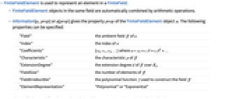
- FiniteFieldElement 用于表示 FiniteField 中的元素.
- 同一域中的 FiniteFieldElement 对象通过算术运算自动合并.
- Information[a,prop] 或 a[prop] 给出 FiniteFieldElement 对象 a 的属性 prop. 可以指定以下属性:
-
"Field" a 的环境域 ff "Index" a 的索引 "Coefficients" {c0,c1,c2,…},其中 a=c0+c1θ+c2θ2+… "Characteristic" ff 的特征 p "ExtensionDegree" ff 在
上的扩张度 d"FieldSize" ff 的元素数目 "FieldIrreducible" 用于构造域 ff 的多项式函数 f "ElementRepresentation" "Polynomial" 或者 "Exponential" - MinimalPolynomial[a,x] 给出
中在 a 处为零的次数最小的一元多项式. - MultiplicativeOrder 给出非零有限域元素的乘法阶.
- PolynomialGCD、Factor、Expand、PolynomialQuotientRemainder 和 Resultant 等多项式运算可用于具有有限域元素系数的多项式. Together 和 Cancel 可用于具有有限域元素系数的有理函数.
- 线性代数运算,如 Det、Inverse、RowReduce、NullSpace、MatrixRank 和 LinearSolve 等,可用于具有有限域元素的矩阵.
- Solve 和 Reduce 可用于求解有限域上的方程组.
范例
打开所有单元 关闭所有单元基本范例 (3)
ℱ = FiniteField[17, 3]{a, b} = {FiniteFieldElement[ℱ, {1, 2, 3}], FiniteFieldElement[ℱ, 123]}{a, b} = {ℱ[{1, 2, 3}], ℱ[123]}(a ^ 2 + 2b) / (5a b - 7){a, b} = {FiniteField[3, 5][121], FiniteField[3, 5][212]}PolynomialRemainder[x ^ 5 - 1, a x ^ 3 + b x + a b, x]a = FiniteFieldElement[FiniteField[7, 5], 777]AtomQ[a]a[{"Field", "Index", "Coefficients"}]范围 (16)
表示和属性 (4)
ℱ = FiniteField[97, 4]a = FiniteFieldElement[ℱ, {1, 2, 3, 4}]ℱ[{1, 2, 3, 4}] === aAtomQ[a]a["Coefficients"]a["Field"]b = FiniteFieldElement[ℱ, 1234]ℱ[123] === bb["Index"]b["Field"]b[{"Characteristic", "ExtensionDegree", "FieldIrreducible"}]使用 Information 提取属性:
Information[ℱ, {"FieldSize", "ElementRepresentation"}]a - aa / aℱ = FiniteField[7, 3, "Exponential"]θ = ℱ[2]q = θ["FieldSize"]And@@Table[ℱ[ind] == θ ^ (ind - 1), {ind, q - 1}]θ - θθ / θa = θ ^ 77a["Coefficients"]%.{1, θ, θ ^ 2}ℱ = FiniteField[2, 100];
ℱ[2 ^ 99]ℱ = FiniteField[NextPrime[2 ^ 100], 3];
ℱ[123]算术 (3)
ℱ = FiniteField[3, 6];
{a, b} = {ℱ[123], ℱ[432]}{a + b, a - b, a b, a / b, a ^ 321}{a ^ (1 / 3), Sqrt[a]}Sqrt[b]ℱ = FiniteField[19, 3];
a = ℱ[123]{a + 5, 7a}a + 7 / 8a + 2 / 19使用 Element 决定哪些有理数可以用域元素标识:
{Element[7 / 8, ℱ], Element[2 / 19, ℱ]}ℱ[0] == 0ℱ[1] == 1ℱ = FiniteField[389, 2];
𝒢 = FiniteField[389, 4];ℱ[123] - 𝒢[123]ℋ = FiniteField[389, Information[ℱ, "FieldIrreducible"], "Exponential"];ℱ[123] - ℋ[123]自同构和嵌入 (2)
ℱ = FiniteField[7, 5];
a = ℱ[123]conj = Table[FrobeniusAutomorphism[a, i], {i, 0, 4}]f = MinimalPolynomial[a]f /@ conjFrobeniusAutomorphism[a] == a ^ 7𝒦 = FiniteField[29, 3];
ℱ = FiniteField[29, 6];
emb = FiniteFieldEmbedding[𝒦, ℱ]emb[𝒦[123]]{a, b} = {𝒦[345], 𝒦[678]};emb[a + b] == emb[a] + emb[b]emb[a b] == emb[a]emb[b]有限域上的多项式 (2)
ℱ = FiniteField[11, 3];
f = ℱ[1]x ^ 2 + ℱ[2]x + ℱ[3];
g = ℱ[12]x ^ 5 + ℱ[21]x + ℱ[33];
h = ℱ[321]x ^ 3 + ℱ[27]x ^ 2 + ℱ[53]x + ℱ[19];fg = Expand[f g]gh = Expand[g h]gcd = PolynomialGCD[fg, gh]Cancel[gcd / g]{q, r} = PolynomialQuotientRemainder[g, h, x]Expand[g - q h - r]Factor[h]Resultant[f, g, x]Expand[(f y + g z)(h z + 1)]Factor[%]Discriminant[f y ^ 2 + g y + h, y]ℱ = FiniteField[29, 3];
𝒢 = FiniteField[29, 6];
ℰ = FiniteFieldEmbedding[ℱ, 𝒢];Factor[ℱ[12]x ^ 2 + ℱ[34]x + ℱ[56]]Factor[ℱ[12]x ^ 2 + ℱ[34]x + ℱ[56], Extension -> ℰ]有限域上的线性代数 (4)
a = (| | | |
| ---------------------------------------------------------------------------------------- | ---------------------------------------------------------------------------------------- | --------------------------------------------------------------------------------------- |
| FiniteFieldElement[FiniteField[29, 2 + 15*#1 + 2*#1^2 + #1^4 & , "Polynomial"], {12}] | FiniteFieldElement[FiniteField[29, 2 + 15*#1 + 2*#1^2 + #1^4 & , "Polynomial"], {23}] | FiniteFieldElement[FiniteField[29, 2 + 15*#1 + 2*#1^2 + #1^4 & , "Polynomial"], {5, 1}] |
| FiniteFieldElement[FiniteField[29, 2 + 15*#1 + 2*#1^2 + #1^4 & , "Polynomial"], {16, 1}] | FiniteFieldElement[FiniteField[29, 2 + 15*#1 + 2*#1^2 + #1^4 & , "Polynomial"], {27, 1}] | FiniteFieldElement[FiniteField[29, 2 + 15*#1 + 2*#1^2 + #1^4 & , "Polynomial"], {9, 2}] |
| FiniteFieldElement[FiniteField[29, 2 + 15*#1 + 2*#1^2 + #1^4 & , "Polynomial"], {20, 2}] | FiniteFieldElement[FiniteField[29, 2 + 15*#1 + 2*#1^2 + #1^4 & , "Polynomial"], {2, 3}] | FiniteFieldElement[FiniteField[29, 2 + 15*#1 + 2*#1^2 + #1^4 & , "Polynomial"], {3, 3}] |);b = (| | |
| ----------------------------------------------------------------------------------------- | ----------------------------------------------------------------------------------------- |
| FiniteFieldElement[FiniteField[29, 2 + 15*#1 + 2*#1^2 + #1^4 & , "Polynomial"], {7, 4}] | FiniteFieldElement[FiniteField[29, 2 + 15*#1 + 2*#1^2 + #1^4 & , "Polynomial"], {2, 8}] |
| FiniteFieldElement[FiniteField[29, 2 + 15*#1 + 2*#1^2 + #1^4 & , "Polynomial"], {26, 11}] | FiniteFieldElement[FiniteField[29, 2 + 15*#1 + 2*#1^2 + #1^4 & , "Polynomial"], {21, 15}] |
| FiniteFieldElement[FiniteField[29, 2 + 15*#1 + 2*#1^2 + #1^4 & , "Polynomial"], {16, 19}] | FiniteFieldElement[FiniteField[29, 2 + 15*#1 + 2*#1^2 + #1^4 & , "Polynomial"], {11, 23}] |);
a.b//MatrixFormMatrixPower[a, 123456789]//MatrixForma = (| | | |
| ---------------------------------------------------------------------------------------- | ---------------------------------------------------------------------------------------- | --------------------------------------------------------------------------------------- |
| FiniteFieldElement[FiniteField[29, 2 + 15*#1 + 2*#1^2 + #1^4 & , "Polynomial"], {12}] | FiniteFieldElement[FiniteField[29, 2 + 15*#1 + 2*#1^2 + #1^4 & , "Polynomial"], {23}] | FiniteFieldElement[FiniteField[29, 2 + 15*#1 + 2*#1^2 + #1^4 & , "Polynomial"], {5, 1}] |
| FiniteFieldElement[FiniteField[29, 2 + 15*#1 + 2*#1^2 + #1^4 & , "Polynomial"], {16, 1}] | FiniteFieldElement[FiniteField[29, 2 + 15*#1 + 2*#1^2 + #1^4 & , "Polynomial"], {27, 1}] | FiniteFieldElement[FiniteField[29, 2 + 15*#1 + 2*#1^2 + #1^4 & , "Polynomial"], {9, 2}] |
| FiniteFieldElement[FiniteField[29, 2 + 15*#1 + 2*#1^2 + #1^4 & , "Polynomial"], {20, 2}] | FiniteFieldElement[FiniteField[29, 2 + 15*#1 + 2*#1^2 + #1^4 & , "Polynomial"], {2, 3}] | FiniteFieldElement[FiniteField[29, 2 + 15*#1 + 2*#1^2 + #1^4 & , "Polynomial"], {3, 3}] |);
Det[a]Inverse[a]//MatrixForm%.a//MatrixFormCharacteristicPolynomial[a, x]CoefficientList[%, x].(MatrixPower[a, #]& /@ Range[0, 3])//MatrixFormc = (| | | | |
| -------------------------------------------------------------------------------------------- | -------------------------------------------------------------------------------------------- | ------------------------------------------------------------------------------------------- | --------------------------------------------------------------------------------------------- |
| FiniteFieldElement[FiniteField[29, 2 + 15*#1 + 2*#1^2 + #1^4 & , "Polynomial"], {16, 13, 1}] | FiniteFieldElement[FiniteField[29, 2 + 15*#1 + 2*#1^2 + #1^4 & , "Polynomial"], {25, 22, 2}] | FiniteFieldElement[FiniteField[29, 2 + 15*#1 + 2*#1^2 + #1^4 & , "Polynomial"], {5, 3, 4}] | FiniteFieldElement[FiniteField[29, 2 + 15*#1 + 2*#1^2 + #1^4 & , "Polynomial"], {14, 12, 5}] |
| FiniteFieldElement[FiniteField[29, 2 + 15*#1 + 2*#1^2 + #1^4 & , "Polynomial"], {23, 21, 6}] | FiniteFieldElement[FiniteField[29, 2 + 15*#1 + 2*#1^2 + #1^4 & , "Polynomial"], {3, 2, 8}] | FiniteFieldElement[FiniteField[29, 2 + 15*#1 + 2*#1^2 + #1^4 & , "Polynomial"], {2, 11, 9}] | FiniteFieldElement[FiniteField[29, 2 + 15*#1 + 2*#1^2 + #1^4 & , "Polynomial"], {27, 16, 10}] |);MatrixRank[c]NullSpace[c]//MatrixFormc.Transpose[%]//MatrixFormRowReduce[c]//MatrixForma = (| | | |
| ---------------------------------------------------------------------------------------- | ---------------------------------------------------------------------------------------- | --------------------------------------------------------------------------------------- |
| FiniteFieldElement[FiniteField[29, 2 + 15*#1 + 2*#1^2 + #1^4 & , "Polynomial"], {12}] | FiniteFieldElement[FiniteField[29, 2 + 15*#1 + 2*#1^2 + #1^4 & , "Polynomial"], {23}] | FiniteFieldElement[FiniteField[29, 2 + 15*#1 + 2*#1^2 + #1^4 & , "Polynomial"], {5, 1}] |
| FiniteFieldElement[FiniteField[29, 2 + 15*#1 + 2*#1^2 + #1^4 & , "Polynomial"], {16, 1}] | FiniteFieldElement[FiniteField[29, 2 + 15*#1 + 2*#1^2 + #1^4 & , "Polynomial"], {27, 1}] | FiniteFieldElement[FiniteField[29, 2 + 15*#1 + 2*#1^2 + #1^4 & , "Polynomial"], {9, 2}] |
| FiniteFieldElement[FiniteField[29, 2 + 15*#1 + 2*#1^2 + #1^4 & , "Polynomial"], {20, 2}] | FiniteFieldElement[FiniteField[29, 2 + 15*#1 + 2*#1^2 + #1^4 & , "Polynomial"], {2, 3}] | FiniteFieldElement[FiniteField[29, 2 + 15*#1 + 2*#1^2 + #1^4 & , "Polynomial"], {3, 3}] |);b = (| | |
| ----------------------------------------------------------------------------------------- | ----------------------------------------------------------------------------------------- |
| FiniteFieldElement[FiniteField[29, 2 + 15*#1 + 2*#1^2 + #1^4 & , "Polynomial"], {7, 4}] | FiniteFieldElement[FiniteField[29, 2 + 15*#1 + 2*#1^2 + #1^4 & , "Polynomial"], {2, 8}] |
| FiniteFieldElement[FiniteField[29, 2 + 15*#1 + 2*#1^2 + #1^4 & , "Polynomial"], {26, 11}] | FiniteFieldElement[FiniteField[29, 2 + 15*#1 + 2*#1^2 + #1^4 & , "Polynomial"], {21, 15}] |
| FiniteFieldElement[FiniteField[29, 2 + 15*#1 + 2*#1^2 + #1^4 & , "Polynomial"], {16, 19}] | FiniteFieldElement[FiniteField[29, 2 + 15*#1 + 2*#1^2 + #1^4 & , "Polynomial"], {11, 23}] |);
(x = LinearSolve[a, b])//MatrixForma.x === b{l, u, p, cn} = LUDecomposition[a]l.u === p.ax == LinearSolve[u, LinearSolve[l, p.b]]有限域上的方程 (1)
ℱ = FiniteField[7, 5];Solve[x ^ 5 + ℱ[123]x == ℱ[127], x]Reduce[x ^ 9 + 5 x + 3 == 0, x, ℱ]Solve[ℱ[123]x + ℱ[234]y == ℱ[345] && ℱ[321]x + ℱ[432]y == ℱ[543], {x, y}]Reduce[ℱ[1234]x + ℱ[2345]y + ℱ[3456]z == ℱ[4567] && ℱ[1]x + ℱ[2]y + ℱ[3]z == ℱ[4], {x, y, z}]Solve[x ^ 2 + y ^ 2 == 3 && x ^ 5 + y ^ 5 == 5, {x, y}, ℱ]Reduce[ℱ[123]x ^ 2 + ℱ[234]y ^ 3 + ℱ[345]z ^ 4 == ℱ[456] && ℱ[21]x + ℱ[32]y ^ 2 + ℱ[43]z ^ 3 == ℱ[54] && x y z == ℱ[1], {x, y, z}]FindInstance[x ^ 2 + y ^ 2 + z ^ 2 == 21, {x, y, z}, ℱ]FindInstance[ℱ[321]x ^ 3 + ℱ[432]y ^ 3 + ℱ[543]z ^ 3 == ℱ[654] && x ^ 2 == ℱ[333]y z + ℱ[111], {x, y, z}, 3]Resolve[Exists[z, ℱ[111]x + ℱ[222]y + ℱ[333]z == ℱ[444] && ℱ[555]x + ℱ[666]y + ℱ[777]z == ℱ[888]]]𝒦 = FiniteField[2, 5];Resolve[Exists[{y, z}, 𝒦[1]x ^ 2 + 𝒦[2]y ^ 3 + 𝒦[3]z ^ 4 == 𝒦[4] && 𝒦[5]x ^ 4 + 𝒦[6]y ^ 3 + 𝒦[7]z ^ 2 == 𝒦[8] && x y z != 𝒦[0]]]应用 (8)
执行纠错码.
汉明码将
位消息编码为
位序列,并且可以纠正至多一个错误:
m = 5;
n = 2 ^ m - 1;
k = n - m;令
为使用指数元素表示法的具有
个元素的有限域,令
是用于构造
的不可约多项式,令
为
的生成器:
ℱ = FiniteField[2, m, "Exponential"];
f = Information[ℱ, "FieldIrreducible"][x];
θ = ℱ[{0, 1}]encode[kbits_] := PadRight[Mod[CoefficientList[f(kbits.x ^ Range[0, k - 1]), x], 2], n]msg = Table[RandomInteger[], {k}]enc = encode[msg]t[nbits_, x_] := nbits.x ^ Range[0, n - 1]t[enc, θ]err = ReplaceAt[enc, e_ :> 1 - e, RandomInteger[{1, n}]]t[err, θ]correct[nbits_] :=
With[{ep = t[nbits, θ]},
If[ep == 0,
nbits,
ReplaceAt[nbits, e_ :> 1 - e, ep["Index"]]]]correct[err] === encdecode[nbits_] := PadRight[CoefficientList[PolynomialQuotient[nbits.x ^ Range[0, n - 1], f, x, Modulus -> 2], x], k]当接收到的消息没有错误或有一个错误时,解码后的消息是正确的:
decode[correct[enc]] === msgdecode[correct[err]] === msg为任意质数幂
构造
个正交的
阶拉丁方阵.
阶拉丁方阵是一个
数组,其中每一行和每一列都包含恰好
个元素中的每个元素一次. 如果通过并置两个数组形成的
个数对都不同,则称这对拉丁方阵是正交的:
q = 9;
ℱ = FiniteField[3, 2];
squares = Table[Table[(ℱ[k]ℱ[i - 1] + ℱ[j - 1])["Index"] + 1, {i, q}, {j, q}], {k, q - 1}];
MatrixForm /@ squareslatinQ[a_] := Union[Sort /@ Join[a, Transpose[a]]] === {Range[q]}latinQ /@ squaresorthogonalQ[a_, b_] := Length[Union[Transpose[{Flatten[a], Flatten[b]}]]] == q ^ 2orthogonalQ@@@Subsets[squares, {2}]如果
时,和
都是不同的,那么一个有限的整数集合
是一个西顿集合(Sidon set). 对于质幂
,在
中构造一个
个整数的西顿集合:
sidon[q_] :=
Module[{ff, g},
ff = FiniteField[q ^ 2, "Exponential"];
g = ff[2];Prepend[Select[Range[q ^ 2 - 1], Mod[(g ^ # - g)["Index"] - 1, q + 1] == 0&], 1]]q = 27;
a = sidon[q]Length[a] == qsums = Join@@Table[a[[i]] + a[[j]], {j, q}, {i, j}];Length[sums] == Length[Union[sums]] == q(q + 1) / 2对于有
个字母的字母表,阶
的 de Bruijn 序列是字母表中
个字母的循环序列
,使得
个字母的每个序列作为
的子序列恰好出现一次. 为一个有
个字母的字母表构造一个阶数为
的 de Bruijn 序列,取质幂
:
deBruijn[q_, n_] :=
Module[{f1, f2, emb, s, p},
f1 = FiniteField[q, "Exponential"];
f2 = FiniteField[q ^ n, "Exponential"];
emb = FiniteFieldEmbedding[f1, f2];
s = FiniteFieldIndex[emb["Projection"][FromFiniteFieldIndex[Range[q ^ n - 1], f2]]];
p = SequencePosition[s, Table[0, {n - 1}]][[1, 1]];
Insert[s, 0, p]]q = 8;n = 3;
s = deBruijn[q, n]验证对于一个有
个字母的字母表,
是阶数为
的 de Bruijn 序列:
Sort[Partition[s, n, 1, 1]] === Tuples[Range[0, q - 1], n]如果
的所有项为
或
且
,则
矩阵
是哈达玛(Hadamard)矩阵. 为任意素幂
构建一个阶数为
的哈达玛矩阵,其中
:
ξ[e_] := If[Head[Sqrt[e]] === FiniteFieldElement, 1, -1]
h[0, _, _] := 1
h[_, 0, _] := 1
h[i_, j_, ff_] := If[i == j, -1, ξ[ff[j - 1] - ff[i - 1]]]q = 7 ^ 3;
ℱ = FiniteField[7, 3];
(H = Table[h[i, j, ℱ], {i, 0, q}, {j, 0, q}])//MatrixPlotUnion[Flatten[H]]H.Transpose[H] === (q + 1)IdentityMatrix[q + 1]实现高级加密标准(AES)算法中使用的 Rijndael S 盒步骤. 第一部分称为 Nyberg S 盒,使用
中的乘法逆:
F256 = FiniteField[2, # ^ 8 + # ^ 4 + # ^ 3 + # + 1&]NybergSbox[byte_] := Piecewise[{{(F256[byte] ^ (-1))["Index"], byte != 0}}, 0]F2 = FiniteField[2];
a = Map[F2, {{1, 0, 0, 0, 1, 1, 1, 1}, {1, 1, 0, 0, 0, 1, 1, 1}, {1, 1, 1, 0, 0, 0, 1, 1}, {1, 1, 1, 1, 0, 0, 0, 1}, {1, 1, 1, 1, 1, 0, 0, 0}, {0, 1, 1, 1, 1, 1, 0, 0}, {0, 0, 1, 1, 1, 1, 1, 0}, {0, 0, 0, 1, 1, 1, 1, 1}}, {2}];
b = F2 /@ {1, 1, 0, 0, 0, 1, 1, 0};
affine[byte_] := FromDigits[Reverse[FiniteFieldIndex[a.Reverse[IntegerDigits[byte, 2, 8]] + b]], 2]ForwardSbox[byte_] := affine[NybergSbox[byte]]tohex[byte_] := StringJoin@@(FromCharacterCode[If[# <= 9, # + 48, # + 87]]& /@ IntegerDigits[byte, 16, 2])Table[tohex[ForwardSbox[16i + j]], {i, 0, 15}, {j, 0, 15}]//MatrixFormainv = Inverse[a];
affineinv[byte_] := FromDigits[Reverse[FiniteFieldIndex[ainv.(Reverse[IntegerDigits[byte, 2, 8]] - b)]], 2]InverseSbox[byte_] := NybergSbox[affineinv[byte]]Table[tohex[InverseSbox[16i + j]], {i, 0, 15}, {j, 0, 15}]//MatrixForm(InverseSbox /@ ForwardSbox /@ Range[0, 255]) === Range[0, 255]使用 2049 位素数实现 Diffie–Hellman 公钥密码系统:
p = 32317006071311007300714876688669951960444102669715484032130345427524655138867890893197201411522913463688717960921898019494119559150490921095088152386448283120630877367300996091750197750389652106796057638384067568276792218642619756161838094338476170470581645852036305042887575891541065808607552399123930385521914333389668342420684974786564569494856176035326322058077805659331026192708460314150258592864177116725943603718461857357598351152301645904403697613233287231227125684710820209725157101726931323469678542580656697935045997268352998638215525166389437335543602135433229604645318478604952148193555853611059596248443;
ℱ = FiniteField[p];g = ℱ[PrimitiveRoot[p]]SeedRandom[1234];a = RandomInteger[{2, p - 2}]g1 = g ^ ab = RandomInteger[{2, p - 2}]m = RandomInteger[{1, 2 ^ 2048}]e = m g1 ^ bg2 = g ^ bd = e / g2 ^ ad["Index"] == mp = 179769313486231590772930519078902473361797697894230657273430081157732675805500963132708477322407536021120113879871393357658789768814416622492847430639474124377767893424865485276302219601246094119453082952085005768838150682342462881473913110540827237163350510684586298239947245938479716304835356329624224143009;
Zp = FiniteField[p];
g = Zp[PrimitiveRoot[p]]SeedRandom[1234];
h = RandomInteger[{2, p - 1}];
c = g ^ h信息
的签名是一对
小于
并使得
的正整数. 计算签名需要知道秘密整数
:
signature[m_] :=
Module[{k, a, b, d, r, s},
k = 2;
While[GCD[k, p - 1] != 1, k++];
{d, {a, b}} = ExtendedGCD[k, p - 1];
r = (g ^ k)["Index"];
s = Mod[a(m - h r), p - 1];
{r, s}]verify[{r_, s_}, m_] := g ^ m == c ^ r Zp[r] ^ sm = RandomInteger[{1, p - 1}];
{r, s} = signature[m]verify[{r, s}, m]属性和关系 (9)
ℱ = FiniteField[7, 10]Information[ℱ, "FieldSize"] == 7 ^ 10ℱ = FiniteField[11, 3];
{a, b} = {ℱ[123], ℱ[456]}{(a + b) ^ 11, a ^ 11 + b ^ 11}因此映射
是一个域自同构,称为 FrobeniusAutomorphism:
FrobeniusAutomorphism[a] == a ^ 11ℱ = FiniteField[109, 5];
θ = ℱ[{0, 1}]f = Information[ℱ, "FieldIrreducible"]f[θ]使用 FrobeniusAutomorphism 求
的剩余根:
Table[FrobeniusAutomorphism[θ, k], {k, 4}]f /@ %使用 MinimalPolynomial 求有限域元素的最小多项式:

ℱ = FiniteField[11, 6];
a = ℱ[1234]MinimalPolynomial[a, x]MinimalPolynomial[a, x, 2]ℱ = FiniteField[3, 5];
q = Information[ℱ, "FieldSize"]Union[x ^ q - x /. Table[{x -> ℱ[i]}, {i, 0, q - 1}]]Expand[Product[x - ℱ[i], {i, 0, q - 1}]]Coefficient[%, x, 1] == -1ℱ = FiniteField[73, 6];
f = 9x ^ 6 + 54x ^ 2 + 42x + 11使用 IrreduciblePolynomialQ 与 Modulusp 验证在
上的不可约性:
IrreduciblePolynomialQ[f, Modulus -> 73]使用 Factor 与 Extensionℱ 验证 f 是
上线性因子的乘积:
Factor[f, Extension -> ℱ]使用 MultiplicativeOrder 求有限域元素的乘法阶:
ℱ = FiniteField[1009, 7];
a = ℱ[1234]MultiplicativeOrder[a]a ^ %使用 FiniteField[p,1] 在质数域
上计算:
ℱ = FiniteField[19, 1];ℱ[12] ℱ[7] + ℱ[3]与使用 Mod 获得的结果进行比较:
Mod[12 7 + 3, 19]Discriminant[ℱ[4]x ^ 3 + ℱ[5]a x + ℱ[11], x]与使用 Modulus 选项获得的结果进行比较:
Discriminant[4x ^ 3 + 5a x + 11, x, Modulus -> 19]使用 FromFiniteFieldIndex 来获取指定索引的域元素:
FromFiniteFieldIndex[{123, 234, 345}, FiniteField[19, 2]]FiniteFieldIndex 给出了域元素的索引:
FiniteFieldIndex[%]文本
Wolfram Research (2023),FiniteFieldElement,Wolfram 语言函数,https://reference.wolfram.com/language/ref/FiniteFieldElement.html (更新于 2024 年).
CMS
Wolfram 语言. 2023. "FiniteFieldElement." Wolfram 语言与系统参考资料中心. Wolfram Research. 最新版本 2024. https://reference.wolfram.com/language/ref/FiniteFieldElement.html.
APA
Wolfram 语言. (2023). FiniteFieldElement. Wolfram 语言与系统参考资料中心. 追溯自 https://reference.wolfram.com/language/ref/FiniteFieldElement.html 年
BibTeX
@misc{reference.wolfram_2026_finitefieldelement, author="Wolfram Research", title="{FiniteFieldElement}", year="2024", howpublished="\url{https://reference.wolfram.com/language/ref/FiniteFieldElement.html}", note=[Accessed: 13-August-2026]}
BibLaTeX
@online{reference.wolfram_2026_finitefieldelement, organization={Wolfram Research}, title={FiniteFieldElement}, year={2024}, url={https://reference.wolfram.com/language/ref/FiniteFieldElement.html}, note=[Accessed: 13-August-2026]}