Wolfram 语言与系统参考资料中心

InfiniteLine

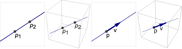
InfiniteLine[{p₁,p₂}]

表示经过点 p₁ 和 p₂ 的无限长直线.

InfiniteLine[p,v]

表示经过点 p，方向为 v 的无限长直线.

范例

打开所有单元关闭所有单元

基本范例 (3)

二维 InfiniteLine：

Wolfram Language code: Graphics[InfiniteLine[{0, 0}, {1, 1}], Frame -> True]

三维：

Wolfram Language code: Graphics3D[InfiniteLine[{0, 0, 0}, {1, 2, 3}]]

无限长直线的几种不同样式：

Wolfram Language code: ℛ = InfiniteLine[{0, 0}, {1, 1}];

Wolfram Language code:

{Graphics[{Red, ℛ}, Frame -> True], Graphics[{Thick, Red, ℛ}, Frame -> True], Graphics[{Thick, Red, Dashed, ℛ}, Frame -> True]}

判断某点是否在无限长直线上：

Wolfram Language code: ℛ = InfiniteLine[{0, 0}, {1, 1}];

Wolfram Language code: {RegionMember[ℛ, {2, 2}], RegionMember[ℛ, {2, 3}]}

范围 (19)

图形 (8)

规范 (3)

定义一条包含方向为的 InfiniteLine：

Wolfram Language code:

ill = Graphics[{PointSize[Medium], Point[{{1, 1}}], Arrowheads[Medium], Thick, Arrow[{{1, 1}, {3, 2}}]}, PlotRange -> {{0, 4}, {0, 3}}, Frame -> True];

Wolfram Language code: Show[ill, Graphics[InfiniteLine[{1, 1}, {2, 1}]]]

定义同样的，经过和的直线：

Wolfram Language code: ill = Graphics[{PointSize[Medium], Point[{{1, 1}, {3, 2}}]}, PlotRange -> {{0, 4}, {0, 3}}, Frame -> True];

Wolfram Language code: Show[ill, Graphics[InfiniteLine[{{1, 1}, {3, 2}}]]]

定义一条三维无限长直线，包含并沿着方向：

Wolfram Language code:

ill = Graphics3D[{PointSize[Medium], Point[{{1, 1, 1}}], Arrowheads[Medium], Thick, Arrow[{{1, 1, 1}, {2, 3, 4}}]}, PlotRange -> {{0, 5}, {0, 5}, {0, 5}}, Axes -> True];

Wolfram Language code: Show[ill, Graphics3D[InfiniteLine[{1, 1, 1}, {1, 2, 3}]]]

用点和来定义同一条无限长直线：

Wolfram Language code:

ill = Graphics3D[{PointSize[Medium], Point[{{1, 1, 1}, {2, 3, 4}}]}, PlotRange -> {{0, 5}, {0, 5}, {0, 5}}, Axes -> True];

Wolfram Language code: Show[ill, Graphics3D[InfiniteLine[{{1, 1, 1}, {2, 3, 4}}]]]

方向不同的无限长直线：

Wolfram Language code: Table[Graphics[InfiniteLine[{0, 0}, {Cos[θ], Sin[θ]}], ImageSize -> Tiny, PlotLabel -> θ], {θ, 0, π, π / 4}]

样式 (4)

以缩放尺寸规定的粗细：

Wolfram Language code: Table[Graphics[{Thickness[i], InfiniteLine[{{0, 0}, {2, 1}}]}], {i, {.005, .05, .1}}]

以打印机点规定的粗细：

Wolfram Language code: Table[Graphics[{AbsoluteThickness[i], InfiniteLine[{{0, 0}, {2, 1}}]}], {i, {1, 5, 10}}]

无限长直线还可以渲染为虚线或点划线：

Wolfram Language code: Table[Graphics[{Dashing[i], InfiniteLine[{{0, 0}, {2, 1}}]}], {i, {Tiny, Small, Medium, Large}}]

Wolfram Language code: Table[Graphics[{d, InfiniteLine[{{0, 0}, {2, 1}}]}], {d, {Dotted, Dashed, DotDashed}}]

可以用着色指令来指定无限长直线的颜色：

Wolfram Language code: Table[Graphics[{c, InfiniteLine[{{0, 0}, {2, 1}}]}], {c, {Red, Green, Blue, Yellow}}]

组合不同指令来指定无限长直线的样式：

Wolfram Language code: Graphics[{Thick, Blue, Dashed, InfiniteLine[{{0, 0}, {2, 1}}]}]

坐标 (1)

点和矢量可以是 Dynamic 表达式：

Wolfram Language code: DynamicModule[{θ = 0}, {Slider[Dynamic[θ], {0, Pi}], Graphics[InfiniteLine[{0, 0}, Dynamic[{Cos[θ], Sin[θ]}]]]}]

区域 (11)

嵌入维度是顶点的维数：

Wolfram Language code: RegionEmbeddingDimension[InfiniteLine[{{x0, y0}, {x1, y1}}]]

Wolfram Language code: RegionEmbeddingDimension[InfiniteLine[{x, y, z}, {a, b, c}]]

几何维度是区域自身的维度：

Wolfram Language code: RegionDimension[InfiniteLine[{{x0, y0}, {x1, y1}}]]

Wolfram Language code: RegionDimension[InfiniteLine[{x, y, z}, {a, b, c}]]

判断某点是否为该区域的成员：

Wolfram Language code: RegionMember[InfiniteLine[{{0, 0, 0}, {1, 1, 1}}], {2, 2, 2}]

Wolfram Language code: RegionMember[InfiniteLine[{1, 1}, {2, 2}], {0, -1}]

获取成为该区域成员的条件：

Wolfram Language code: RegionMember[InfiniteLine[{{x0, y0}, {x1, y1}}], {x, y}]

无限长直线是无界的：

Wolfram Language code: ℛ = InfiniteLine[{{0, 0}, {1, 1}}];

Wolfram Language code: BoundedRegionQ[ℛ]

给出区域范围：

Wolfram Language code: RegionBounds[ℛ]

InfiniteLine 的度量为无限大：

Wolfram Language code: ℛ = InfiniteLine[{{0, 0}, {1, 1}}];

Wolfram Language code: RegionMeasure[ℛ]

Wolfram Language code: RegionCentroid[ℛ]

到一个点的距离：

Wolfram Language code: ℛ = InfiniteLine[{{2, 2}, {3, 3}}];

Wolfram Language code: RegionDistance[ℛ, {0, 1}]

画出到区域的距离：

Wolfram Language code:

{Plot3D[Evaluate@RegionDistance[ℛ, {x, y}], {x, -2, 2}, {y, -2, 2}, MeshFunctions -> {#3&}, Mesh -> 5], ContourPlot[Evaluate[RegionDistance[ℛ, {x, y}]], {x, -3, 3}, {y, -3, 3}, Contours -> {{0.5, Red}, {1, Green}, {1.5, Blue}}]}

到一个点的有向距离：

Wolfram Language code: ℛ = InfiniteLine[{{2, 2}, {3, 3}}];

Wolfram Language code: SignedRegionDistance[ℛ, {0, -1}]

到最近的点的距离：

Wolfram Language code: Plot3D[SignedRegionDistance[ℛ, {x, y}], {x, -2, 2}, {y, -2, 2}, MeshFunctions -> {#3&}, Mesh -> 5]

区域中最近的点：

Wolfram Language code: ℛ = InfiniteLine[{{2, 2}, {3, 3}}];

Wolfram Language code: RegionNearest[ℛ, {5, 6}]

可视化最近的点：

Wolfram Language code:

pts = Table[{1, 2} + 5{Cos[k 2 π / 16], Sin[k 2π / 16]}, {k, 0., 15}];
nst = RegionNearest[ℛ, #]& /@ pts;

Wolfram Language code:

Legended[Graphics[{{Gray, ℛ}, {Thin, Gray, Line[Transpose[{pts, nst}]]}, {Red, Point[pts]}, {Blue, Point[nst]}}], PointLegend[{Red, Blue}, {"start", "nearest"}]]

在无限长直线上积分：

Wolfram Language code: ℛ = InfiniteLine[{{0, 0}, {1, 1}}];

Wolfram Language code: Integrate[Exp[-x y], {x, y}∈ℛ]

在无限长直线上最优化：

Wolfram Language code: ℛ = InfiniteLine[{0, 0}, {1, 1}];

Wolfram Language code: Minimize[{(x y - 1)^2 + 3, {x, y}∈ℛ}, {x, y}]

在无限长直线上求解方程：

Wolfram Language code: ℛ = InfiniteLine[{0, 0, 0}, {1, 2, 3}];

Wolfram Language code: Solve[x^2 + y^2 + z^2 == 1 && {x, y, z}∈ℛ, {x, y, z}]

Wolfram Language code: Graphics3D[{{Opacity[0.5], Sphere[]}, ℛ, {Red, PointSize[Large], Point[{x, y, z} /. %]}}]

应用 (17)

生成和平行排列的直线：

Wolfram Language code: lines = Table[InfiniteLine[{0, y}, {1, 1}], {y, 5}];

Wolfram Language code: Graphics[lines, PlotRange -> {{-6, 6}, {0, 6}}]

可视化渐近线：

Wolfram Language code: asym = InfiniteLine[{0, 0}, {1, 1}];

Wolfram Language code: Plot[(x ^ 2 + x + 1/x + 1), {x, -1, 7}, Epilog -> {Red, Dashed, asym}, PlotRange -> 7]

Wolfram Language code: ParametricPlot[{t + Cos[14 t] / t, t + Sin[14 t] / t}, {t, 0.01, 10}, Epilog -> {Red, Dashed, asym}]

将直线的截距式转换为 InfiniteLine：

Wolfram Language code:

a = 2;
b = 3;

Wolfram Language code: ir = ImplicitRegion[(x/a) + (y/b) == 1, {x, y}];

Wolfram Language code: il = InfiniteLine[{{a, 0}, {0, b}}];

可视化直线：

Wolfram Language code: Table[RegionPlot[r, PlotRange -> {{0, 3}, {0, 3}}], {r, {ir, il}}]

将直线的点斜式转换为 InfiniteLine：

Wolfram Language code:

m = 2 / 3;
{x0, y0} = {1, 2};

Wolfram Language code: ir = ImplicitRegion[y - y0 == m(x - x0), {x, y}];

Wolfram Language code: il = InfiniteLine[{x0, y0}, {1, m}];

可视化直线：

Wolfram Language code: Table[RegionPlot[r, PlotRange -> {{0, 3}, {0, 3}}], {r, {ir, il}}]

将直线的斜截式转换为 InfiniteLine：

Wolfram Language code:

m = 2 / 3;
b = 1;

Wolfram Language code: ir = ImplicitRegion[y == m x + b, {x, y}];

Wolfram Language code: il = InfiniteLine[{0, b}, {1, m}];

可视化直线：

Wolfram Language code: Table[RegionPlot[r, PlotRange -> {{0, 3}, {0, 3}}], {r, {ir, il}}]

将直线的两点式转换为 InfiniteLine：

Wolfram Language code:

{x0, y0} = {0, 2};
{x1, y1} = {3, 1};

Wolfram Language code: ir = ImplicitRegion[y - y0 == (y1 - y0/x1 - x0)(x - x0), {x, y}];

Wolfram Language code: il = InfiniteLine[{{x0, y0}, {x1, y1}}];

可视化直线：

Wolfram Language code: Table[RegionPlot[r, PlotRange -> {{0, 3}, {0, 3}}], {r, {ir, il}}]

将直线的参数式转换为 InfiniteLine：

Wolfram Language code:

a = 2;
b = 3;
{x0, y0} = {1, 2};

Wolfram Language code: pr = ParametricRegion[{x0 + a t, y0 + b t}, {t}];

Wolfram Language code: il = InfiniteLine[{{x0, y0}, {x0 + a, y0 + b}}];

可视化直线：

Wolfram Language code: Table[RegionPlot[r, PlotRange -> {{0, 3}, {0, 3}}], {r, {pr, il}}]

参数式曲线 f[u] 的切线为 InfiniteLine[f[u],f'[u]]. 计算参数式曲线的切线：

Wolfram Language code: f1[u_] := {Cos[u], Sin[u]};

Wolfram Language code:

c1 = ParametricPlot[f1[u], {u, 0, 2π}];
t1 = With[{u = π / 4}, Graphics[InfiniteLine[f1[u], f1'[u]]]];

Wolfram Language code: Show[c1, t1, PlotRange -> {{-2, 2}, {-2, 2}}]

计算参数式曲线的切线：

Wolfram Language code: f2[u_] := {Cos[u], Sin[u], u / 10};

Wolfram Language code:

c2 = ParametricPlot3D[f2[t], {t, 0, 20}];
t2 = With[{u = 4}, Graphics3D[InfiniteLine[f2[u], f2'[u]]]];

Wolfram Language code: Show[c2, t2, PlotRange -> {{-2, 2}, {-2, 2}, All}]

计算 InfiniteLine[{0,0},{1,1}] 和 InfiniteLine[{{0,1},{1,0}}] 的交点：

Wolfram Language code:

line1 = InfiniteLine[{0, 0}, {1, 1}];
line2 = InfiniteLine[{{0, 1}, {1, 0}}];

Wolfram Language code: sol = Solve[{x, y}∈line1∧{x, y}∈line2, {x, y}]

画出图形：

Wolfram Language code: Graphics[{{Lighter[Blue, 0.5], line1, line2}, {Red, Point[{x, y} /. sol]}}, Axes -> True, ImageSize -> Small]

计算 InfiniteLine[{0,0},{1,1}] 和 Circle[{0,0},1] 的交点：

Wolfram Language code:

line = InfiniteLine[{0, 0}, {1, 1}];
circle = Circle[{0, 0}, 1];

Wolfram Language code: sol = Solve[{x, y}∈line∧{x, y}∈circle, {x, y}]

画出图形：

Wolfram Language code: Graphics[{{Lighter[Blue, 0.5], line, circle}, {Red, Point[{x, y} /. sol]}}, ImageSize -> Small]

计算五条随机直线两两相交的交点：

Wolfram Language code: lines = InfiniteLine /@ RandomReal[1, {5, 2, 2}];

利用 BooleanCountingFunction 来表示恰好满足两个条件的情况：

Wolfram Language code: sol = NSolve[{x, y}∈BooleanRegion[BooleanCountingFunction[{2}, 5], lines], {x, y}]

画出图形：

Wolfram Language code: Graphics[{{Lighter[Blue, 0.5], lines}, {Red, PointSize[Medium], Point[{x, y} /. sol]}}]

计算 InfiniteLine[{{-1,1,1},{1,1,1}}] 和 InfinitePlane[{{2,0,0},{0,2,0},{0,0,2}}] 的交点：

Wolfram Language code:

line = InfiniteLine[{{-1, 1, 1}, {1, 1, 1}}];
plane = InfinitePlane[{{2, 0, 0}, {0, 2, 0}, {0, 0, 2}}];

Wolfram Language code: sol = Solve[{{x, y, z}∈line, {x, y, z}∈plane}, {x, y, z}]

画出图形：

Wolfram Language code:

Graphics3D[{{Opacity[0.5], line, plane}, {Red, PointSize[Large], Point[{x, y, z} /. sol]}}, Axes -> True, PlotRange -> {{-2, 2}, {-2, 2}, {-2, 2}}]

计算 InfiniteLine[{{-1,1,1},{1,1,1}}] 和 Sphere[{0,0,0},3] 的交点：

Wolfram Language code:

line = InfiniteLine[{{-1, 1, 1}, {1, 1, 1}}];
sphere = Sphere[{0, 0, 0}, 3];

Wolfram Language code: sol = Solve[{{x, y, z}∈line, {x, y, z}∈sphere}, {x, y, z}]

画出图形：

Wolfram Language code: Graphics3D[{{Opacity[0.5], line, sphere}, {Red, PointSize[Large], Point[{x, y, z} /. sol]}}, PlotRangePadding -> 0.5]

计算 InfiniteLine[{{-1,1/3,1/2},{1,1/3,1/2}}] 和 Tetrahedron[{{0,0,0},{1,0,0},{0,1,0},{0,0,1}}] 的表面的交点：

Wolfram Language code:

line = InfiniteLine[{{-1, 1 / 3, 1 / 2}, {1, 1 / 3, 1 / 2}}];
tet = RegionBoundary@Tetrahedron[{{0, 0, 0}, {1, 0, 0}, {0, 1, 0}, {0, 0, 1}}];

Wolfram Language code: sol = Solve[{x, y, z}∈RegionIntersection[line, tet], {x, y, z}]

画出图形：

Wolfram Language code:

Graphics3D[{{Opacity[0.5], line, Tetrahedron[{{0, 0, 0}, {1, 0, 0}, {0, 1, 0}, {0, 0, 1}}]}, {Red, PointSize[Medium], Point[{x, y, z} /. sol]}}, PlotRangePadding -> 0.2]

在 Histogram 上标出 Mean：

Wolfram Language code: data = RandomVariate[NormalDistribution[1, 9], 200];

Wolfram Language code: h = Histogram[data];

Wolfram Language code: m = Graphics[{Dashed, Red, InfiniteLine[{Mean[data], 0}, {0, 1}]}];

Wolfram Language code: Show[h, m]

可视化 RotationTransform 的旋转轴：

Wolfram Language code:

v = {4, 2, -5};
p = {2, 2, 3 / 2};

Wolfram Language code: axis = InfiniteLine[p, v];

Wolfram Language code: rt[θ_] := RotationTransform[θ, v, p];

Wolfram Language code: g = Graphics3D[Table[{GeometricTransformation[Sphere[], rt[θ]]}, {θ, 0, 2Pi, 2Pi / 8}], Boxed -> False];

Wolfram Language code: Show[g, Graphics3D[{Thick, Blue, Dashed, axis}]]

计算三角形的高线：

Wolfram Language code: {a, b, c} = {{0, 0}, {3, 0}, {-1, 2}};

Wolfram Language code: base = InfiniteLine[{a, b}];

Wolfram Language code: foot = RegionNearest[base, c];

Wolfram Language code: altitude = Line[{c, foot}];

用红色标出高线：

Wolfram Language code:

Graphics[{{LightBlue, Triangle[{a, b, c}]}, {Thick, Darker@LightBlue, base}, {PointSize@Medium, Red, Point[{c, foot}]}, {Dashed, Red, altitude}}]

属性和关系 (5)

InfiniteLine[{p₁,p₂}] 等价于 InfiniteLine[p₁,p₂-p₁]：

Wolfram Language code:

Subscript[ℛ, 1] = InfiniteLine[{{1, 0}, {2, 2}}];
Subscript[ℛ, 2] = InfiniteLine[{1, 0}, {1, 2}];

Wolfram Language code: RegionEqual[Subscript[ℛ, 1], Subscript[ℛ, 2]]

在二维空间，InfiniteLine[p,v] 等价于 Hyperplane[Cross[v],p]：

Wolfram Language code: Subscript[ℛ, 1] = InfiniteLine[{1, 2}, {1, 1}];

Wolfram Language code: Subscript[ℛ, 2] = Hyperplane[Cross[{1, 1}], {1, 2}];

Wolfram Language code: RegionEqual[Subscript[ℛ, 1], Subscript[ℛ, 2]]

ParametricRegion 可以表示任意 InfiniteLine：

Wolfram Language code:

Subscript[ℛ, 1] = ParametricRegion[{1, 2} + t{3, 4}, {t}];
Subscript[ℛ, 2] = InfiniteLine[{1, 2}, {3, 4}];

Wolfram Language code: RegionEqual[Subscript[ℛ, 1], Subscript[ℛ, 2]]

ImplicitRegion 可以表示任意 InfiniteLine：

Wolfram Language code:

Subscript[ℛ, 1] = ImplicitRegion[y - x == 1, {x, y}];
Subscript[ℛ, 2] = InfiniteLine[{{1, 2}, {3, 4}}];

Wolfram Language code: RegionEqual[Subscript[ℛ, 1], Subscript[ℛ, 2]]

InfiniteLine 是 ConicHullRegion 的一个特例：

Wolfram Language code: pts = {{1, 2}, {3, 4}};

Wolfram Language code: RegionEqual[ConicHullRegion[pts], InfiniteLine[pts]]

巧妙范例 (2)

随意排列的直线：

Wolfram Language code: Graphics[Table[{Hue[RandomReal[]], InfiniteLine[RandomReal[1, {2, 2}]]}, {50}]]

Wolfram Language code: Graphics3D[Table[{Hue[RandomReal[]], InfiniteLine[RandomReal[1, {2, 3}]]}, {100}], BoxRatios -> 1]

有序排列的直线：

Wolfram Language code: Graphics[Table[InfiniteLine[{0, 0}, {Cos[θ], Sin[θ]}], {θ, 0., π, π / 50}]]

Wolfram Language code: Graphics[Table[InfiniteLine[{Cos[θ], Sin[θ]}, {-Sin[θ], Cos[θ]}], {θ, 0, 2π, π / 20}], PlotRange -> 2]

Top

更多学习资源

技术支持

数据科学、金融与商业

工程

科学与技术

教育科技

教育举措

开始

提高你的技能

与我们合作

成人教育计划

青少年教育计划

欢迎阅读

InfiniteLine

更多信息

范例

基本范例 (3)

范围 (19)

图形 (8)

规范 (3)

样式 (4)

坐标 (1)

区域 (11)

应用 (17)

属性和关系 (5)

巧妙范例 (2)

文本

CMS

APA

BibTeX

BibLaTeX

InfiniteLine

更多信息

范例

基本范例 (3)

范围 (19)

图形 (8)

规范 (3)

样式 (4)

坐标 (1)

区域 (11)

应用 (17)

属性和关系 (5)

巧妙范例 (2)

参见

相关指南

历史

文本

CMS

APA

BibTeX

BibLaTeX