

LineIntegrate
LineIntegrate[f,{x,y,…}∈curve]
関数 f[x,y,…]の curve 上のスカラー線積分を計算する.
LineIntegrate[{p,q,…},{x,y,…}∈curve]
ベクトル関数上の{p[x,y,…],q[x,y,…],…}のベクトル線積分を計算する.
詳細とオプション
- 線積分は,曲線積分としても知られている.
- スカラー線積分は曲線に沿ってスカラー関数を積分する.この積分は,主に,曲線の長さ,質量,電荷を計算する.
- ベクトル線積分は,ベクトル関数が曲線に沿って接線方向に移動するときにベクトル関数によって行われる仕事量を計算するために使われる.主なベクトル関数には,力場,電場,流体速度場がある.
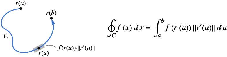
- curve に沿った関数 f のスカラー線積分
 は以下で与えられる.
 - ここで,
![TemplateBox[{{{r, ^, {(, ', )}}, (, u, )}}, Norm]](Files/LineIntegrate.ja/2.png "TemplateBox[{{{r, ^, {(, ', )}}, (, u, )}}, Norm]") はパラメトリック曲線セグメントの測定値である.
はパラメトリック曲線セグメントの測定値である. - スカラー線積分は curve のパラメータ化や向きには依存しない.任意次元のRegionQオブジェクトを curve として使うことができる.
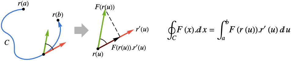
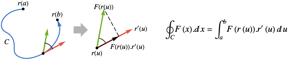
- curve に沿った関数 F のベクトル線積分
 は以下で与えられる.
 - ここで,
 は成分の接線方向の成分だけが積分されるためのベクトル関数
  の接線方向への射影である.
 - ベクトル線積分は曲線のパラメータ化には依存しないが,曲線の向きには依存する.
- 曲線の向きは曲線上の接線ベクトル場
 によって与えられる.
 - パラメトリック曲線ParametricRegion[{r1[u],…,rn[u]},…]について,接線ベクトル場
 は ∂ur[u]であるとみなされる.
 - 次は,
 における特殊曲線と仮定される接線の向きである.
 -

Line[{p1,p2,…}] 向きは点 p1,p2等が与えられた順による 
HalfLine[{p1,p2}]
HalfLine[p,v]向きは p1から p2または v の方向 
InfiniteLine[{p1,p2}]
InfiniteLine[p,v]向きは p1から p2または v の方向 
Circle[p,r] 向きは反時計回り - 次は,
 における特殊曲線と仮定される接線の向きである.
 -

Line[{p1,p2,…}] 向きは点 p1,p2等が与えられた順による 
HalfLine[{p1,p2}]
HalfLine[p,v]向きは p1から p2または v の方向 
InfiniteLine[{p1,p2}]
InfiniteLine[p,v]向きは p1から p2または v の方向 - 次は,
 における特殊曲線と仮定される接線の向きである.
 -

Line[{p1,p2,…}] 向きは与えられた点の順序による 
HalfLine[{p1,p2}]
HalfLine[p,v]向きは p1 から p2 へ 向きは v によって与えられる 
InfiniteLine[{p1,p2}]
InfiniteLine[p,v]向きは p1 から p2 へ 向きは v によって与えられる - curve に沿った座標はVectorSymbolを使って指定できる. »
- 次は,使用可能なオプションである.
-
Assumptions $Assumptions パラメータについての仮定 Direction Automatic 曲線の向き GenerateConditions Automatic パラメータについての仮定を含む答を生成するかどうか WorkingPrecision Automatic 内部計算精度 - LineIntegrateは,入力に厳密ではない数量が含まれる場合は記号メソッドと数値メソッドを組み合せて使う.
例題
すべて開く すべて閉じる例 (7)
LineIntegrate[2x, {x, y}∈Circle[{0, 0}, 1, {0, Pi / 2}]]LineIntegrate[{x * y, x - y}, {x, y}∈Line[{{0, 0}, {1, 1}}]]LineIntegrate[{x ^ 2 y z, 3x y, y ^ 2}, {x, y, z}∈ParametricRegion[{Cos[t], Sin[t], t}, {{t, 0, Pi / 2}}]]f = y ^ 2;reg = ParametricRegion[{{t ^ (5 / 2), t}, 0 <= t <= 2}, {t}];
Show[ContourPlot[f, {x, 0, 8}, {y, 0, 2}], ...]LineIntegrate[f, {x, y}∈reg]f = {x + 2y, x ^ 2};reg = Line[{{0, 0}, {2, 3 / 2}, {3, 0}}];VectorPlot[f, {x, 0, 3}, {y, 0, 2}, ...]LineIntegrate[f, {x, y}∈reg]f = {z ^ 3, x ^ 3, y ^ 3};reg = Line[{{1, 1 / 2, 0}, {3, 2, 2}}];Show[VectorPlot3D[f, {x, 0, 4}, {y, 0, 2}, {z, 0, 2}, Rule[...]], ...]LineIntegrate[f, {x, y, z}∈reg]VectorSymbolを使う:
LineIntegrate[VectorSymbol["x"].VectorSymbol["x"], VectorSymbol["x"]∈Line[{{0, 0}, {0, 1}}]]LineIntegrate[x, x∈Line[{{0, 0}, {0, 1}}]]スコープ (32)
基本的な用法 (4)
f = Exp[x];LineIntegrate[f, {x, y}∈Line[{{0, 0}, {2, 3}}]]f = {x, x - y, z x ^ 2};LineIntegrate[f, {x, y, z}∈ParametricRegion[{Sin[t], t, 2t}, {{t, 0, Pi}}]]LineIntegrate は多くの特殊曲線に使うことができる:
f = {x ^ 2 y, x};reg = Annulus[{0, 0}, {1, 2}, {0, Pi / 4}];LineIntegrate[f, {x, y}∈reg]f = {Log[x], y};reg = ParametricRegion[{2t + 1, t ^ 2}, {{t, 0, 1}}];LineIntegrate[f, {x, y}∈reg]スカラー関数 (11)
f = 2x - 2 y;reg = ParametricRegion[{t, t ^ (3 / 2)}, {{t, 0, 8}}];
Show[ContourPlot[f, {x, 0, 8}, {y, 0, 25}], ...]LineIntegrate[f, {x, y}∈reg]f = 1 / (x + y + 1);reg = Circle[{0, 0}, 1, {0, Pi / 2}];ContourPlot[f, {x, 0, 1}, {y, 0, 1}, Epilog -> reg, ImageSize -> Small]LineIntegrate[f, {x, y}∈reg]f = 1 / (x + 1) - y / 5;reg = ParametricRegion[{3 / 2t ^ 2, 4t}, {{t, -1, 1}}];Show[ContourPlot[f, {x, -1 / 2, 2}, {y, -4, 4}], ...]LineIntegrate[f, {x, y}∈reg]f = x ^ 3 + y + 1;reg = Circle[{1, 2}, 3];ContourPlot[f, {x, -2, 4}, {y, -1, 5}, Epilog -> reg, ImageSize -> Small]LineIntegrate[f, {x, y}∈reg]f = x + y - z;reg = ParametricRegion[{t ^ 3 / 3, Sqrt[2]t ^ 2 / 2, t}, {{t, 0, 1}}];LineIntegrate[f, {x, y, z}∈reg]f = 1 / (x + y + 5);reg = Annulus[{0, 0}, {1, 2}, {0, 3 / 4Pi}];ContourPlot[f, {x, -2, 4}, {y, -1, 5}, ...]LineIntegrate[f, {x, y}∈reg]f = Exp[Abs[x - y]];reg = Line[{{0, 0}, {1, 2}, {0, 1}, {0, 0}}];ContourPlot[f, {x, 0, 1}, {y, 0, 2}, Epilog -> reg, AspectRatio -> Automatic]LineIntegrate[f, {x, y}∈reg]f = 2 x y;reg = Circle[{0, 0}, {1, 1 / Sqrt[2]}];ContourPlot[f, {x, -1, 1}, {y, -1, 1}, Epilog -> reg, ImageSize -> Small]LineIntegrate[f, {x, y}∈reg]f = x / 2 + y ^ 2;reg = ParametricRegion[{6Cos[t] - Cos[6t], 6Sin[t] - Sin[6t]}, {{t, 0, 2Pi}}];Show[ContourPlot[f, {x, -10, 10}, {y, -10, 10}], RegionPlot[reg, BoundaryStyle -> Blue], ImageSize -> Small]LineIntegrate[f, {x, y}∈reg]f = ArcTan[(y / x) ^ 2];reg = Circle[{0, 0}, 4];
ContourPlot[f, {x, -4, 4}, {y, -4, 4}, Epilog -> reg, ImageSize -> Small]LineIntegrate[f, {x, y}∈reg]f = x - y;reg = Disk[{0, 0}, 3, {0, 3Pi / 4}];
ContourPlot[f, {x, -3, 3}, {y, -1, 5}, ...]LineIntegrate[f, {x, y}∈reg]ベクトル関数 (12)
f = {2x, x, 1};reg = ParametricRegion[{Sin[t], Cos[t], t}, {{t, 0, 2Pi}}];Show[VectorPlot3D[f, {x, -1, 1}, {y, -1, 1}, {z, 0, 7}, ...], ...]LineIntegrate[f, {x, y, z}∈reg]f = {Sin[x], y};reg = ParametricRegion[{t ^ 2, t ^ 3}, {{t, 0, 1}}];Show[VectorPlot[f, {x, 0, 1}, {y, 0, 1}, Rule[...]], ...]LineIntegrate[f, {x, y}∈reg]f = {x * (x ^ 2 + y ^ 2), y * (x ^ 2 + y ^ 2)};reg = Circle[{0, 0}, 1, {0, Pi / 2}];VectorPlot[f, {x, 0, 1}, {y, 0, 1}, ...]LineIntegrate[f, {x, y}∈reg]f = {Sqrt[x ^ 2 + y ^ 2], Sqrt[x + y]};reg = Line[{{0, 0}, {2, 2}, {4, 0}}];VectorPlot[f, {x, -1, 5}, {y, -1, 3}, ...]LineIntegrate[f, {x, y}∈reg]f = {x, x ^ 2 y ^ 2, 0};reg = ParametricRegion[{Cos[t] ^ 2, Cos[t]Sin[t], Sqrt[Cos[t](1 - Cos[t])]}, {{t, 0, 2Pi}}];Show[VectorPlot3D[f, {x, -1, 1}, {y, -1, 1}, {z, 0, 1}, Rule[...]], ...]LineIntegrate[f, {x, y, z}∈reg]f = {x + y, y + z, z + x};reg = ParametricRegion[{Sin[t] ^ 2 / Sqrt[2] + Cos[t] ^ 2, (1 - 1 / Sqrt[2])Cos[t]Sin[t], Sin[t] / Sqrt[2]}, {{t, 0, 2Pi}}];Show[VectorPlot3D[f, {x, 0, 1}, {y, -1, 1}, {z, -1, 1}, ...], ...]LineIntegrate[f, {x, y, z}∈reg]f = {x, x y};reg = Circle[{0, 0}, {2, 1}, {0, Pi}];VectorPlot[f, {x, -2, 2}, {y, -1 / 2, 3 / 2}, ...]LineIntegrate[f, {x, y}∈reg]f = {x ^ 2, x ^ 2, y ^ 2};reg = ParametricRegion[{(2 + Cos[3t])Cos[t], (2 + Cos[3t])Sin[t], Sin[3t]}, {{t, 0, 2Pi}}];Show[VectorPlot3D[f, {x, -3, 3}, {y, -3, 3}, {z, -1, 1}, ...], ...]LineIntegrate[f, {x, y, z}∈reg]f = {(y - 1) ^ 2z, x ^ 2y, 2x y};reg = ParametricRegion[{Cos[t], Sin[t] / 2, Sin[t] / 2}, {{t, 0, Pi}}];Show[VectorPlot3D[f, {x, -1, 1}, {y, -1, 1}, {z, -1, 1}, Rule[...]], ...]LineIntegrate[f, {x, y, z}∈reg]f = {x ^ 2, 1 / 3, z ^ 2};reg = ParametricRegion[{2 / (1 + t ^ 2), 3t, 2t / (1 + t ^ 2)}, {{t, -10, 10}}];Show[VectorPlot3D[f, {x, 0, 2}, {y, -30, 30}, {z, -1, 1}, ...], ...]LineIntegrate[f, {x, y, z}∈reg]f = {y ^ 2, Sin[y]};reg = Circle[{0, 1}, {Sqrt[2], 1}];VectorPlot[f, {x, -2, 2}, {y, 0, 2}, ...]LineIntegrate[f, {x, y}∈reg]f = {x y, x ^ 2t z, y t, z t};LineIntegrate[f, {x, y, z, t}∈Line[{{0, 0, 0, 0}, {1, 2, 3, 4}}]]特殊曲線 (4)
f = Sqrt[x] * y ^ 4;reg = Circle[{0, 0}, 4, {-Pi / 2, Pi / 2}];ContourPlot[f, {x, 0, 4}, {y, -4, 4}, ...]LineIntegrate[f, {x, y}∈reg]f = {0, x ^ 2};reg = Disk[{0, 0}, 1, {0, Pi / 2}];VectorPlot[f, {x, 0, 1}, {y, 0, 1}, ...]LineIntegrate[f, {x, y}∈reg]f = {1 / (x + y), -1 / (x + y)};reg = Line[{{1, 0}, {0, 1}, {-1, 0}, {0, -1}, {1, 0}}];VectorPlot[f, {x, -1, 1}, {y, -1, 1}, ...]LineIntegrate[f, {x, y}∈reg]f = {-y, x};reg = Annulus[{0, 0}, {1, 2}, {0, Pi / 4}];VectorPlot[f, {x, 0, 2}, {y, 0, 2}, ...]LineIntegrate[f, {x, y}∈reg]パラメトリック曲線 (1)
オプション (5)
Assumptions (1)
オプションAssumptionsはパラメータに使うことができる:
LineIntegrate[Exp[-a x], {x, y}∈ParametricRegion[{2t, 3t}, {{t, 0, Infinity}}]]LineIntegrate[Exp[-a x], {x, y}∈ParametricRegion[{2t, 3t}, {{t, 0, Infinity}}], Assumptions -> Re[a] > 0]Direction (1)
閉じた円形経路についてのデフォルトのDirectionは反時計回りである:
f = {-x ^ 2y, y ^ 2};reg = Circle[];VectorPlot[f, {x, -1, 1}, {y, -1, 1}, ...]LineIntegrate[f, {x, y}∈reg]LineIntegrate[f, {x, y}∈reg, Direction -> "Anticlockwise"]Directionオプションを使って時計回りの方向を選ぶことができる:
LineIntegrate[f, {x, y}∈reg, Direction -> "Clockwise"]GenerateConditions (1)
LineIntegrateは記号パラメータで使うことができる:
LineIntegrate[Exp[-a x], {x, y}∈ParametricRegion[{2t, 3t}, {{t, 0, Infinity}}]]LineIntegrate[Exp[-a x], {x, y}∈ParametricRegion[{2t, 3t}, {{t, 0, Infinity}}], GenerateConditions -> False]WorkingPrecision (2)
WorkingPrecisionが指定されているなら数値結果が与えられる:
LineIntegrate[1, {x, y}∈Circle[]]LineIntegrate[1, {x, y}∈Circle[], WorkingPrecision -> 16]LineIntegrate[{-y, 0.567x}, {x, y}∈Line[{{0, 0}, {2, 4}}]]アプリケーション (27)
大学の微積分 (10)

f = x y ^ 2 z ^ 3;reg = Line[{{-1, 3, 1}, {1, 7, 3}}];LineIntegrate[f, {x, y, z}∈reg]f = {x Sin[y], y Cos[z], z Sin[x]};reg = ParametricRegion[{Cos[t], Sin[t] ^ 2, -Cos[t]}, {{t, 0, Pi}}];LineIntegrate[f, {x, y, z}∈reg]
ρ = x ^ 2y ^ 2;reg = Circle[{0, 0}, 1];LineIntegrate[ρ, {x, y}∈reg]
f = {x - y ^ 3, y - z ^ 3, z - x ^ 3};reg = Line[{{0, 0, 0}, {1, 2, 3}}];LineIntegrate[f, {x, y, z}∈reg]f = {Cos[x], Sin[y]};reg = Line[{{0, 0}, {3, 0}, {3, 3}, {0, 3}, {0, 0}}];LineIntegrate[f, {x, y}∈reg]f = {x ^ 2, y ^ 2};reg = ParametricRegion[{t, t ^ 2}, {{t, 0, 1}}];LineIntegrate[f, {x, y}∈reg]

f = {x ^ 2, y};reg = ParametricRegion[{t - Sin[t], 1 - Cos[t]}, {{t, 0, 2Pi}}];LineIntegrate[f, {x, y}∈reg]f = {x + y, x ^ 2};LineIntegrate[f, {x, y}∈Circle[]]
f = {x ^ 2 / (x ^ 2 + y ^ 2), (y ^ 2 - x ^ 2) / (x ^ 2 + y ^ 2)};LineIntegrate[f, {x, y}∈Circle[{0, 0}, R]]f = {Exp[Sin[x ^ 2]], Exp[Sqrt[x ^ 2 + y ^ 2]]};reg = ParametricRegion[{Sin[t ^ 2], Cos[t] ^ 3}, {{t, 0, 2Pi}}];LineIntegrate[f, {x, y}∈reg, WorkingPrecision -> 16]長さ (3)
LineIntegrate[1, {x, y}∈Circle[]]reg = ParametricRegion[{(2Cos[t] - Cos[2t]), (2Sin[t] - Sin[2t])}, {{t, 0, 2Pi}}];RegionPlot[reg, ImageSize -> Small]LineIntegrate[1, {x, y}∈reg]長さはRegionMeasureを使っても計算できる:
RegionMeasure[reg]reg = ParametricRegion[{Cos[t] ^ 3, Sin[t] ^ 3}, {{t, 0, 2Pi}}];RegionPlot[reg, ImageSize -> Small]LineIntegrate[1, {x, y}∈reg]面積 (5)


LineIntegrate[{-y / 2, x / 2}, {x, y}∈Circle[{0, 0}, {a, b}]]線積分を使って計算した,レム二スケート 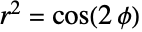 の右側ループの面積:
f = {-y / 2, x / 2};reg = ParametricRegion[{Sqrt[Cos[2ϕ]]Cos[ϕ], Sqrt[Cos[2ϕ]]Sin[ϕ]}, {{ϕ, -Pi / 4, Pi / 4}}];Show[VectorPlot[f, {x, 0, 1}, {y, -1 / 2, 1 / 2}, ...], ...]LineIntegrate[f, {x, y}∈reg]

reg = ParametricRegion[{(R + r)Cos[t] - r Cos[(R + r) / r * t], (R + r)Sin[t] - r Sin[(R + r) / r * t]}, {{t, 0, 2Pi}}];LineIntegrate[{-y / 2, x / 2}, {x, y}∈reg, Assumptions -> R == k * r && k∈Integers]reg = ParametricRegion[{(2Cos[t] - Cos[2t]), (2Sin[t] - Sin[2t])}, {{t, 0, 2Pi}}];RegionPlot[reg, ImageSize -> Small]LineIntegrate[{-y / 2, x / 2}, {x, y}∈reg]reg = ParametricRegion[{Cos[t] ^ 3, Sin[t] ^ 3}, {{t, 0, 2Pi}}];RegionPlot[reg, ImageSize -> Small]LineIntegrate[{-y / 2, x / 2}, {x, y}∈reg]力の働き (4)
オブジェクトが直線上を移動するときに重力によってなされる仕事:
f = {0, 0, -m g};LineIntegrate[f, {x, y, z}∈Line[{{x1, y1, z1}, {x2, y2, z2}}]]電荷密度  の帯電無限ワイヤの電場で電荷
  が{1,1,0}から{2,2,0}に変化するときに電力によってなされる仕事:
f = {(λ * q * x/2Pi Subscript[ϵ, 0](x ^ 2 + y ^ 2)), (λ * q * y/2Pi Subscript[ϵ, 0](x ^ 2 + y ^ 2)), 0};LineIntegrate[f, {x, y, z}∈Line[{{1, 1, 0}, {2, 2, 0}}]]楕円の4分の1をたどったときに原点に向かって弾力によってなされる仕事:
f = {-k x, -k y};reg = Circle[{0, 0}, {a, b}, {0, Pi / 2}];LineIntegrate[f, {x, y}∈reg]電荷  の電場で電荷
  が
が  軸に沿って
軸に沿って  から無限に動くときの弾力の仕事:
f = {(Q * q * x/4π Subscript[ϵ, 0](x ^ 2 + y ^ 2 + z ^ 2) ^ (3 / 2)), (Q * q * y/4π Subscript[ϵ, 0](x ^ 2 + y ^ 2 + z ^ 2) ^ (3 / 2)), (Q * q * z/4π Subscript[ϵ, 0](x ^ 2 + y ^ 2 + z ^ 2) ^ (3 / 2))};reg = ParametricRegion[{Subscript[x, 0] + t, 0, 0}, {{t, 0, Infinity}}];LineIntegrate[f, {x, y, z}∈reg, Assumptions -> Subscript[x, 0] > 0]重心 (2)


reg = Disk[{0, 0}, {1, 1}, {0, Pi}];m = LineIntegrate[λ, {x, y}∈reg]
(1 / m) * LineIntegrate[λ * x, {x, y}∈reg]
(1 / m) * LineIntegrate[λ * y, {x, y}∈reg]
reg = ParametricRegion[{Cos[t], Sin[t], t / 10}, {{t, 0, 6Pi}}];ParametricPlot3D[{Cos[t], Sin[t], t / 10}, {t, 0, 6Pi}, ImageSize -> Small]
LineIntegrate[(y ^ 2 + z ^ 2) * ρ, {x, y, z}∈reg]
LineIntegrate[(x ^ 2 + z ^ 2) * ρ, {x, y, z}∈reg]
LineIntegrate[(x ^ 2 + y ^ 2) * ρ, {x, y, z}∈reg]古典的な定理 (3)
ベクトル場は,その線積分が経路ではなく端点の値にのみ依存するなら「保存的」である:
f = {3 x^2 y, x^3};

g = x ^ 3 y;f == Grad[g, {x, y}]スカラー場のすべての傾きは保存的である.例えば,曲線上の  の線積分は以下のようになる:
reg = ParametricRegion[{t ^ 2, Exp[t]}, {{t, 0, 1}}];LineIntegrate[f, {x, y}∈reg]
(g /. {x -> t ^ 2, y -> Exp[t]} /. t -> 1) - (g /. {x -> t ^ 2, y -> Exp[t]} /. t -> 0)
f = {x ^ 4, x * y ^ 2 + 1};LineIntegrate[f, {x, y}∈Line[{{0, 0}, {1, 0}, {0, 1}, {0, 0}}]]これは, が以下のように定義された曲線によって囲まれた領域上の
  の面積分に関連している:
g = D[f[[2]], x] - D[f[[1]], y];Integrate[g, {x, y}∈Triangle[{{0, 0}, {1, 0}, {0, 1}}]]三次元の閉じた線に沿ったベクトル場  の線積分は以下のようになる:
f = {-y + x y ^ 2, x, z};reg = ParametricRegion[{Cos[t], Sin[t], 0}, {{t, 0, 2Pi}}];LineIntegrate[f, {x, y, z}∈reg]これは,曲線を境界として持つ任意の曲面上の  のCurlの面積分に等しい:
reg2 = ParametricRegion[{Cos[t]Cos[p], Cos[t]Sin[p], Sin[t]}, {{p, 0, 2Pi}, {t, 0, Pi / 2}}];SurfaceIntegrate[Curl[f, {x, y, z}], {x, y, z}∈reg2]SurfaceIntegrate[Curl[f, {x, y, z}], {x, y, z}∈ParametricRegion[{r Cos[t], r Sin[t], 0}, {{r, 0, 1}, {t, 0, 2Pi}}]]特性と関係 (5)
記号計算がうまくいかないときはN[LineIntegrate[...]]を適用して数値解を得るとよい:
f = Sin[x + y + z];reg = ParametricRegion[{t ^ 2, t ^ 3, t ^ 4}, {{t, 0, 1}}];LineIntegrate[f, {x, y, z}∈reg]N[LineIntegrate[f, {x, y, z}∈reg]]reg = Line[{{0, 0}, {1, 0}, {1, 1}, {0, 0}}];RegionPlot[reg, ImageSize -> Small]m = LineIntegrate[1, {x, y}∈reg]
1 / m * LineIntegrate[x, {x, y}∈reg]質量の中心はRegionCentroidを使って求めることもできる:
RegionCentroid[reg] -
- 平面の原点を中心とした単位線密度の円形ワイヤの
  軸の周りの慣性モーメントを求める:
reg = ParametricRegion[{Cos[t], Sin[t], 0}, {{t, 0, 2Pi}}];LineIntegrate[(x ^ 2 + y ^ 2), {x, y, z}∈reg]答はMomentOfInertiaを使って計算することもできる:
MomentOfInertia[reg, {0, 0, 0}, {0, 0, 1}]reg = ParametricRegion[{6 Cos[t] - Cos[6 t], 6 Sin[t] - Sin[6 t]}, {{t, 0, 2Pi}}];RegionPlot[reg, ImageSize -> Small]LineIntegrate[1, {x, y}∈reg]ArcLengthを使っても同じ答が得られる:
ArcLength[{6 Cos[t] - Cos[6 t], 6 Sin[t] - Sin[6 t]}, {t, 0, 2Pi}]reg = Circle[{0, 0}, {1 / Sqrt[2], 1 / Sqrt[3]}];LineIntegrate[{-y / 2, x / 2}, {x, y}∈reg]結果はRegionMeasureを使って求められる:
RegionMeasure[Disk[{0, 0}, {1 / Sqrt[2], 1 / Sqrt[3]}]]おもしろい例題 (2)
reg = ParametricRegion[{t, Cosh[t]}, {{t, -1, 1}}];ParametricPlot[{t, Cosh[t]}, {t, -1, 1}, ImageSize -> Small]LineIntegrate[1, {x, y}∈reg]f = {x ^ 2 + y, y ^ 2 + z, z ^ 2 + x};reg = ParametricRegion[{Cos[t]Cos[3t], Cos[t]Sin[3t], Sin[t]}, {{t, 0, 2Pi}}];Show[VectorPlot3D[f, {x, -1, 1}, {y, -1, 1}, {z, -1, 1}, Rule[...]], ...]LineIntegrate[f, {x, y, z}∈reg]テキスト
Wolfram Research (2023), LineIntegrate, Wolfram言語関数, https://reference.wolfram.com/language/ref/LineIntegrate.html (2025年に更新).
CMS
Wolfram Language. 2023. "LineIntegrate." Wolfram Language & System Documentation Center. Wolfram Research. Last Modified 2025. https://reference.wolfram.com/language/ref/LineIntegrate.html.
APA
Wolfram Language. (2023). LineIntegrate. Wolfram Language & System Documentation Center. Retrieved from https://reference.wolfram.com/language/ref/LineIntegrate.html