

LineIntegrate
LineIntegrate[f,{x,y,…}∈curve]
计算函数 f[x,y,…] 在 curve 上的标量线积分.
LineIntegrate[{p,q,…},{x,y,…}∈curve]
计算矢量函数 {p[x,y,…],q[x,y,…],…} 的矢量线积分.
更多信息和选项
- 线积分也称为曲线积分和功积分.
- 标量线积分沿曲线对标量函数进行积分,通常用于计算曲线的长度、质量和电荷.
- 矢量线积分用于计算矢量函数沿曲线在其切线方向移动时所做的功. 典型的矢量函数包括力场、电场和流体速度场.
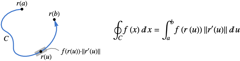
- 函数 f 沿 curve
 的标量线积分由下式给出:
- 其中
 是参数曲线段的度量.
- 标量线积分与 curve 的参数化和方向无关. 任何一维 RegionQ 对象都可以用作 curve.
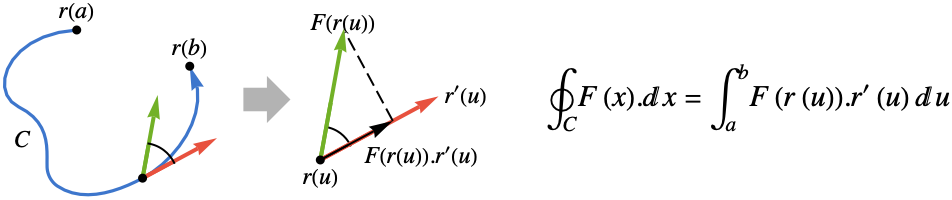
- 函数 F 沿曲线 curve
 的矢量线积分由下式给出:
- 其中
 是矢量函数
 在切线方向上的投影,因此只有切线方向的分量被积分.
- 矢量线积分与曲线的参数化无关,但确实取决于曲线的方向.
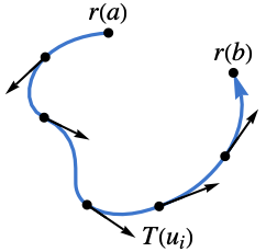
- 曲线的方向由曲线上的切线矢量场
 给出.
- 对于参数曲线 ParametricRegion[{r1[u],…,rn[u]},…],切矢量场
 取作 ∂ur[u].
 中具有假定切线方向的特殊曲线包括:
-

Line[{p1,p2,…}] 方向按照点从 p1 到 p2 等给出的顺序. 
HalfLine[{p1,p2}]
HalfLine[p,v]方向是从 p1 到 p2,或在 v 方向 
InfiniteLine[{p1,p2}]
InfiniteLine[p,v]方向是从 p1 到 p2,或在 v 方向 
Circle[p,r] 方向是逆时针  中具有假定切线方向的特殊曲线包括:
-

Line[{p1,p2,…}] 方向按照点从 p1 到 p2 等给出的顺序 
HalfLine[{p1,p2}]
HalfLine[p,v]方向是从 p1 到 p2,或在 v 方向 
InfiniteLine[{p1,p2}]
InfiniteLine[p,v]方向是从 p1 到 p2,或在 v 方向  中具有假定切线方向的特殊曲线包括:
-

Line[{p1,p2,…}] 方向按照给定的点的顺序 
HalfLine[{p1,p2}]
HalfLine[p,v]方向是从 p1 到 p2 方向由 v 给出 
InfiniteLine[{p1,p2}]
InfiniteLine[p,v]方向是从 p1 到 p2 方向由 v 给出 - 沿 curve 的坐标可以使用 VectorSymbol 指定. »
- 可以给出以下选项:
-
Assumptions $Assumptions 关于参数的假设 Direction Automatic 曲线的方向 GenerateConditions Automatic 是否生成涉及参数条件的答案 WorkingPrecision Automatic 内部计算中使用的精度 - 当输入涉及不精确的数量时,LineIntegrate 使用符号和数值方法的组合.
范例
打开所有单元 关闭所有单元基本范例 (7)
LineIntegrate[2x, {x, y}∈Circle[{0, 0}, 1, {0, Pi / 2}]]LineIntegrate[{x * y, x - y}, {x, y}∈Line[{{0, 0}, {1, 1}}]]LineIntegrate[{x ^ 2 y z, 3x y, y ^ 2}, {x, y, z}∈ParametricRegion[{Cos[t], Sin[t], t}, {{t, 0, Pi / 2}}]]f = y ^ 2;reg = ParametricRegion[{{t ^ (5 / 2), t}, 0 <= t <= 2}, {t}];
Show[ContourPlot[f, {x, 0, 8}, {y, 0, 2}], ...]LineIntegrate[f, {x, y}∈reg]f = {x + 2y, x ^ 2};reg = Line[{{0, 0}, {2, 3 / 2}, {3, 0}}];VectorPlot[f, {x, 0, 3}, {y, 0, 2}, ...]LineIntegrate[f, {x, y}∈reg]f = {z ^ 3, x ^ 3, y ^ 3};reg = Line[{{1, 1 / 2, 0}, {3, 2, 2}}];Show[VectorPlot3D[f, {x, 0, 4}, {y, 0, 2}, {z, 0, 2}, Rule[...]], ...]LineIntegrate[f, {x, y, z}∈reg]使用 VectorSymbol:
LineIntegrate[VectorSymbol["x"].VectorSymbol["x"], VectorSymbol["x"]∈Line[{{0, 0}, {0, 1}}]]LineIntegrate[x, x∈Line[{{0, 0}, {0, 1}}]]范围 (32)
基本用法 (4)
f = Exp[x];LineIntegrate[f, {x, y}∈Line[{{0, 0}, {2, 3}}]]f = {x, x - y, z x ^ 2};LineIntegrate[f, {x, y, z}∈ParametricRegion[{Sin[t], t, 2t}, {{t, 0, Pi}}]]f = {x ^ 2 y, x};reg = Annulus[{0, 0}, {1, 2}, {0, Pi / 4}];LineIntegrate[f, {x, y}∈reg]f = {Log[x], y};reg = ParametricRegion[{2t + 1, t ^ 2}, {{t, 0, 1}}];LineIntegrate[f, {x, y}∈reg]标量函数 (11)
f = 2x - 2 y;reg = ParametricRegion[{t, t ^ (3 / 2)}, {{t, 0, 8}}];
Show[ContourPlot[f, {x, 0, 8}, {y, 0, 25}], ...]LineIntegrate[f, {x, y}∈reg]f = 1 / (x + y + 1);reg = Circle[{0, 0}, 1, {0, Pi / 2}];ContourPlot[f, {x, 0, 1}, {y, 0, 1}, Epilog -> reg, ImageSize -> Small]LineIntegrate[f, {x, y}∈reg]f = 1 / (x + 1) - y / 5;reg = ParametricRegion[{3 / 2t ^ 2, 4t}, {{t, -1, 1}}];Show[ContourPlot[f, {x, -1 / 2, 2}, {y, -4, 4}], ...]LineIntegrate[f, {x, y}∈reg]f = x ^ 3 + y + 1;reg = Circle[{1, 2}, 3];ContourPlot[f, {x, -2, 4}, {y, -1, 5}, Epilog -> reg, ImageSize -> Small]LineIntegrate[f, {x, y}∈reg]f = x + y - z;reg = ParametricRegion[{t ^ 3 / 3, Sqrt[2]t ^ 2 / 2, t}, {{t, 0, 1}}];LineIntegrate[f, {x, y, z}∈reg]f = 1 / (x + y + 5);reg = Annulus[{0, 0}, {1, 2}, {0, 3 / 4Pi}];ContourPlot[f, {x, -2, 4}, {y, -1, 5}, ...]LineIntegrate[f, {x, y}∈reg]f = Exp[Abs[x - y]];reg = Line[{{0, 0}, {1, 2}, {0, 1}, {0, 0}}];ContourPlot[f, {x, 0, 1}, {y, 0, 2}, Epilog -> reg, AspectRatio -> Automatic]LineIntegrate[f, {x, y}∈reg]f = 2 x y;reg = Circle[{0, 0}, {1, 1 / Sqrt[2]}];ContourPlot[f, {x, -1, 1}, {y, -1, 1}, Epilog -> reg, ImageSize -> Small]LineIntegrate[f, {x, y}∈reg]f = x / 2 + y ^ 2;reg = ParametricRegion[{6Cos[t] - Cos[6t], 6Sin[t] - Sin[6t]}, {{t, 0, 2Pi}}];Show[ContourPlot[f, {x, -10, 10}, {y, -10, 10}], RegionPlot[reg, BoundaryStyle -> Blue], ImageSize -> Small]LineIntegrate[f, {x, y}∈reg]f = ArcTan[(y / x) ^ 2];reg = Circle[{0, 0}, 4];
ContourPlot[f, {x, -4, 4}, {y, -4, 4}, Epilog -> reg, ImageSize -> Small]LineIntegrate[f, {x, y}∈reg]f = x - y;reg = Disk[{0, 0}, 3, {0, 3Pi / 4}];
ContourPlot[f, {x, -3, 3}, {y, -1, 5}, ...]LineIntegrate[f, {x, y}∈reg]矢量函数 (12)
f = {2x, x, 1};reg = ParametricRegion[{Sin[t], Cos[t], t}, {{t, 0, 2Pi}}];Show[VectorPlot3D[f, {x, -1, 1}, {y, -1, 1}, {z, 0, 7}, ...], ...]LineIntegrate[f, {x, y, z}∈reg]f = {Sin[x], y};reg = ParametricRegion[{t ^ 2, t ^ 3}, {{t, 0, 1}}];Show[VectorPlot[f, {x, 0, 1}, {y, 0, 1}, Rule[...]], ...]LineIntegrate[f, {x, y}∈reg]f = {x * (x ^ 2 + y ^ 2), y * (x ^ 2 + y ^ 2)};reg = Circle[{0, 0}, 1, {0, Pi / 2}];VectorPlot[f, {x, 0, 1}, {y, 0, 1}, ...]LineIntegrate[f, {x, y}∈reg]f = {Sqrt[x ^ 2 + y ^ 2], Sqrt[x + y]};reg = Line[{{0, 0}, {2, 2}, {4, 0}}];VectorPlot[f, {x, -1, 5}, {y, -1, 3}, ...]LineIntegrate[f, {x, y}∈reg]f = {x, x ^ 2 y ^ 2, 0};reg = ParametricRegion[{Cos[t] ^ 2, Cos[t]Sin[t], Sqrt[Cos[t](1 - Cos[t])]}, {{t, 0, 2Pi}}];Show[VectorPlot3D[f, {x, -1, 1}, {y, -1, 1}, {z, 0, 1}, Rule[...]], ...]LineIntegrate[f, {x, y, z}∈reg]f = {x + y, y + z, z + x};reg = ParametricRegion[{Sin[t] ^ 2 / Sqrt[2] + Cos[t] ^ 2, (1 - 1 / Sqrt[2])Cos[t]Sin[t], Sin[t] / Sqrt[2]}, {{t, 0, 2Pi}}];Show[VectorPlot3D[f, {x, 0, 1}, {y, -1, 1}, {z, -1, 1}, ...], ...]LineIntegrate[f, {x, y, z}∈reg]f = {x, x y};reg = Circle[{0, 0}, {2, 1}, {0, Pi}];VectorPlot[f, {x, -2, 2}, {y, -1 / 2, 3 / 2}, ...]LineIntegrate[f, {x, y}∈reg]f = {x ^ 2, x ^ 2, y ^ 2};reg = ParametricRegion[{(2 + Cos[3t])Cos[t], (2 + Cos[3t])Sin[t], Sin[3t]}, {{t, 0, 2Pi}}];Show[VectorPlot3D[f, {x, -3, 3}, {y, -3, 3}, {z, -1, 1}, ...], ...]LineIntegrate[f, {x, y, z}∈reg]f = {(y - 1) ^ 2z, x ^ 2y, 2x y};reg = ParametricRegion[{Cos[t], Sin[t] / 2, Sin[t] / 2}, {{t, 0, Pi}}];Show[VectorPlot3D[f, {x, -1, 1}, {y, -1, 1}, {z, -1, 1}, Rule[...]], ...]LineIntegrate[f, {x, y, z}∈reg]f = {x ^ 2, 1 / 3, z ^ 2};reg = ParametricRegion[{2 / (1 + t ^ 2), 3t, 2t / (1 + t ^ 2)}, {{t, -10, 10}}];Show[VectorPlot3D[f, {x, 0, 2}, {y, -30, 30}, {z, -1, 1}, ...], ...]LineIntegrate[f, {x, y, z}∈reg]f = {y ^ 2, Sin[y]};reg = Circle[{0, 1}, {Sqrt[2], 1}];VectorPlot[f, {x, -2, 2}, {y, 0, 2}, ...]LineIntegrate[f, {x, y}∈reg]f = {x y, x ^ 2t z, y t, z t};LineIntegrate[f, {x, y, z, t}∈Line[{{0, 0, 0, 0}, {1, 2, 3, 4}}]]特殊曲线 (4)
f = Sqrt[x] * y ^ 4;reg = Circle[{0, 0}, 4, {-Pi / 2, Pi / 2}];ContourPlot[f, {x, 0, 4}, {y, -4, 4}, ...]LineIntegrate[f, {x, y}∈reg]f = {0, x ^ 2};reg = Disk[{0, 0}, 1, {0, Pi / 2}];VectorPlot[f, {x, 0, 1}, {y, 0, 1}, ...]LineIntegrate[f, {x, y}∈reg]f = {1 / (x + y), -1 / (x + y)};reg = Line[{{1, 0}, {0, 1}, {-1, 0}, {0, -1}, {1, 0}}];VectorPlot[f, {x, -1, 1}, {y, -1, 1}, ...]LineIntegrate[f, {x, y}∈reg]f = {-y, x};reg = Annulus[{0, 0}, {1, 2}, {0, Pi / 4}];VectorPlot[f, {x, 0, 2}, {y, 0, 2}, ...]LineIntegrate[f, {x, y}∈reg]参数曲线 (1)
选项 (5)
Assumptions (1)
选项 Assumptions 可用于参数:
LineIntegrate[Exp[-a x], {x, y}∈ParametricRegion[{2t, 3t}, {{t, 0, Infinity}}]]LineIntegrate[Exp[-a x], {x, y}∈ParametricRegion[{2t, 3t}, {{t, 0, Infinity}}], Assumptions -> Re[a] > 0]Direction (1)
闭合圆形路径的默认 Direction 是逆时针方向:
f = {-x ^ 2y, y ^ 2};reg = Circle[];VectorPlot[f, {x, -1, 1}, {y, -1, 1}, ...]LineIntegrate[f, {x, y}∈reg]LineIntegrate[f, {x, y}∈reg, Direction -> "Anticlockwise"]可以使用选项 Direction 选择顺时针方向:
LineIntegrate[f, {x, y}∈reg, Direction -> "Clockwise"]GenerateConditions (1)
LineIntegrate 可以使用符号参数:
LineIntegrate[Exp[-a x], {x, y}∈ParametricRegion[{2t, 3t}, {{t, 0, Infinity}}]]LineIntegrate[Exp[-a x], {x, y}∈ParametricRegion[{2t, 3t}, {{t, 0, Infinity}}], GenerateConditions -> False]WorkingPrecision (2)
如果指定了 WorkingPrecision,则给出数值结果:
LineIntegrate[1, {x, y}∈Circle[]]LineIntegrate[1, {x, y}∈Circle[], WorkingPrecision -> 16]LineIntegrate[{-y, 0.567x}, {x, y}∈Line[{{0, 0}, {2, 4}}]]应用 (27)
大学微积分 (10)

f = x y ^ 2 z ^ 3;reg = Line[{{-1, 3, 1}, {1, 7, 3}}];LineIntegrate[f, {x, y, z}∈reg]f = {x Sin[y], y Cos[z], z Sin[x]};reg = ParametricRegion[{Cos[t], Sin[t] ^ 2, -Cos[t]}, {{t, 0, Pi}}];LineIntegrate[f, {x, y, z}∈reg]
ρ = x ^ 2y ^ 2;reg = Circle[{0, 0}, 1];LineIntegrate[ρ, {x, y}∈reg]
f = {x - y ^ 3, y - z ^ 3, z - x ^ 3};reg = Line[{{0, 0, 0}, {1, 2, 3}}];LineIntegrate[f, {x, y, z}∈reg]f = {Cos[x], Sin[y]};reg = Line[{{0, 0}, {3, 0}, {3, 3}, {0, 3}, {0, 0}}];LineIntegrate[f, {x, y}∈reg]f = {x ^ 2, y ^ 2};reg = ParametricRegion[{t, t ^ 2}, {{t, 0, 1}}];LineIntegrate[f, {x, y}∈reg]

f = {x ^ 2, y};reg = ParametricRegion[{t - Sin[t], 1 - Cos[t]}, {{t, 0, 2Pi}}];LineIntegrate[f, {x, y}∈reg]f = {x + y, x ^ 2};LineIntegrate[f, {x, y}∈Circle[]]
f = {x ^ 2 / (x ^ 2 + y ^ 2), (y ^ 2 - x ^ 2) / (x ^ 2 + y ^ 2)};LineIntegrate[f, {x, y}∈Circle[{0, 0}, R]]f = {Exp[Sin[x ^ 2]], Exp[Sqrt[x ^ 2 + y ^ 2]]};reg = ParametricRegion[{Sin[t ^ 2], Cos[t] ^ 3}, {{t, 0, 2Pi}}];LineIntegrate[f, {x, y}∈reg, WorkingPrecision -> 16]长度 (3)
LineIntegrate[1, {x, y}∈Circle[]]reg = ParametricRegion[{(2Cos[t] - Cos[2t]), (2Sin[t] - Sin[2t])}, {{t, 0, 2Pi}}];RegionPlot[reg, ImageSize -> Small]LineIntegrate[1, {x, y}∈reg]长度也可以用 RegionMeasure 计算:
RegionMeasure[reg]reg = ParametricRegion[{Cos[t] ^ 3, Sin[t] ^ 3}, {{t, 0, 2Pi}}];RegionPlot[reg, ImageSize -> Small]LineIntegrate[1, {x, y}∈reg]面积 (5)


LineIntegrate[{-y / 2, x / 2}, {x, y}∈Circle[{0, 0}, {a, b}]]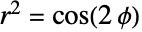
f = {-y / 2, x / 2};reg = ParametricRegion[{Sqrt[Cos[2ϕ]]Cos[ϕ], Sqrt[Cos[2ϕ]]Sin[ϕ]}, {{ϕ, -Pi / 4, Pi / 4}}];Show[VectorPlot[f, {x, 0, 1}, {y, -1 / 2, 1 / 2}, ...], ...]LineIntegrate[f, {x, y}∈reg]

reg = ParametricRegion[{(R + r)Cos[t] - r Cos[(R + r) / r * t], (R + r)Sin[t] - r Sin[(R + r) / r * t]}, {{t, 0, 2Pi}}];LineIntegrate[{-y / 2, x / 2}, {x, y}∈reg, Assumptions -> R == k * r && k∈Integers]reg = ParametricRegion[{(2Cos[t] - Cos[2t]), (2Sin[t] - Sin[2t])}, {{t, 0, 2Pi}}];RegionPlot[reg, ImageSize -> Small]LineIntegrate[{-y / 2, x / 2}, {x, y}∈reg]reg = ParametricRegion[{Cos[t] ^ 3, Sin[t] ^ 3}, {{t, 0, 2Pi}}];RegionPlot[reg, ImageSize -> Small]LineIntegrate[{-y / 2, x / 2}, {x, y}∈reg]力所做的功 (4)
f = {0, 0, -m g};LineIntegrate[f, {x, y, z}∈Line[{{x1, y1, z1}, {x2, y2, z2}}]]在电荷密度为  的带电无限导线的电场中,当电荷
 从 {1,1,0} 移动到 {2,2,0}时,电力所做的功:
f = {(λ * q * x/2Pi Subscript[ϵ, 0](x ^ 2 + y ^ 2)), (λ * q * y/2Pi Subscript[ϵ, 0](x ^ 2 + y ^ 2)), 0};LineIntegrate[f, {x, y, z}∈Line[{{1, 1, 0}, {2, 2, 0}}]]f = {-k x, -k y};reg = Circle[{0, 0}, {a, b}, {0, Pi / 2}];LineIntegrate[f, {x, y}∈reg]电荷  在电荷
 的电场中沿
 轴从
 移动到无穷大时,电力所做的功:
f = {(Q * q * x/4π Subscript[ϵ, 0](x ^ 2 + y ^ 2 + z ^ 2) ^ (3 / 2)), (Q * q * y/4π Subscript[ϵ, 0](x ^ 2 + y ^ 2 + z ^ 2) ^ (3 / 2)), (Q * q * z/4π Subscript[ϵ, 0](x ^ 2 + y ^ 2 + z ^ 2) ^ (3 / 2))};reg = ParametricRegion[{Subscript[x, 0] + t, 0, 0}, {{t, 0, Infinity}}];LineIntegrate[f, {x, y, z}∈reg, Assumptions -> Subscript[x, 0] > 0]质心 (2)


reg = Disk[{0, 0}, {1, 1}, {0, Pi}];m = LineIntegrate[λ, {x, y}∈reg]
(1 / m) * LineIntegrate[λ * x, {x, y}∈reg]
(1 / m) * LineIntegrate[λ * y, {x, y}∈reg]
reg = ParametricRegion[{Cos[t], Sin[t], t / 10}, {{t, 0, 6Pi}}];ParametricPlot3D[{Cos[t], Sin[t], t / 10}, {t, 0, 6Pi}, ImageSize -> Small]
LineIntegrate[(y ^ 2 + z ^ 2) * ρ, {x, y, z}∈reg]
LineIntegrate[(x ^ 2 + z ^ 2) * ρ, {x, y, z}∈reg]
LineIntegrate[(x ^ 2 + y ^ 2) * ρ, {x, y, z}∈reg]经典定理 (3)
如果矢量场的线积分只取决于端点的值,而不取决于路径,那么这个矢量场为保守的(conservative):
f = {3 x^2 y, x^3};

g = x ^ 3 y;f == Grad[g, {x, y}]
reg = ParametricRegion[{t ^ 2, Exp[t]}, {{t, 0, 1}}];LineIntegrate[f, {x, y}∈reg]
(g /. {x -> t ^ 2, y -> Exp[t]} /. t -> 1) - (g /. {x -> t ^ 2, y -> Exp[t]} /. t -> 0)
f = {x ^ 4, x * y ^ 2 + 1};LineIntegrate[f, {x, y}∈Line[{{0, 0}, {1, 0}, {0, 1}, {0, 0}}]]

g = D[f[[2]], x] - D[f[[1]], y];Integrate[g, {x, y}∈Triangle[{{0, 0}, {1, 0}, {0, 1}}]]
f = {-y + x y ^ 2, x, z};reg = ParametricRegion[{Cos[t], Sin[t], 0}, {{t, 0, 2Pi}}];LineIntegrate[f, {x, y, z}∈reg]这等于以曲线为边界的任何曲面上  的 Curl 的曲面积分:
reg2 = ParametricRegion[{Cos[t]Cos[p], Cos[t]Sin[p], Sin[t]}, {{p, 0, 2Pi}, {t, 0, Pi / 2}}];SurfaceIntegrate[Curl[f, {x, y, z}], {x, y, z}∈reg2]SurfaceIntegrate[Curl[f, {x, y, z}], {x, y, z}∈ParametricRegion[{r Cos[t], r Sin[t], 0}, {{r, 0, 1}, {t, 0, 2Pi}}]]属性和关系 (5)
如果符号计算失败,应用 N[LineIntegrate[...]] 获得数值解:
f = Sin[x + y + z];reg = ParametricRegion[{t ^ 2, t ^ 3, t ^ 4}, {{t, 0, 1}}];LineIntegrate[f, {x, y, z}∈reg]N[LineIntegrate[f, {x, y, z}∈reg]]reg = Line[{{0, 0}, {1, 0}, {1, 1}, {0, 0}}];RegionPlot[reg, ImageSize -> Small]m = LineIntegrate[1, {x, y}∈reg]
1 / m * LineIntegrate[x, {x, y}∈reg]也可以使用 RegionCentroid 获得质心:
RegionCentroid[reg]求在  -
 平面上以原点为中心的单位线密度圆线绕
 轴的惯性矩:
reg = ParametricRegion[{Cos[t], Sin[t], 0}, {{t, 0, 2Pi}}];LineIntegrate[(x ^ 2 + y ^ 2), {x, y, z}∈reg]答案也可以用 MomentOfInertia 计算得到:
MomentOfInertia[reg, {0, 0, 0}, {0, 0, 1}]reg = ParametricRegion[{6 Cos[t] - Cos[6 t], 6 Sin[t] - Sin[6 t]}, {{t, 0, 2Pi}}];RegionPlot[reg, ImageSize -> Small]LineIntegrate[1, {x, y}∈reg]使用 ArcLength 可以获得相同的答案:
ArcLength[{6 Cos[t] - Cos[6 t], 6 Sin[t] - Sin[6 t]}, {t, 0, 2Pi}]reg = Circle[{0, 0}, {1 / Sqrt[2], 1 / Sqrt[3]}];LineIntegrate[{-y / 2, x / 2}, {x, y}∈reg]结果可以使用 RegionMeasure 获得:
RegionMeasure[Disk[{0, 0}, {1 / Sqrt[2], 1 / Sqrt[3]}]]巧妙范例 (2)
reg = ParametricRegion[{t, Cosh[t]}, {{t, -1, 1}}];ParametricPlot[{t, Cosh[t]}, {t, -1, 1}, ImageSize -> Small]LineIntegrate[1, {x, y}∈reg]f = {x ^ 2 + y, y ^ 2 + z, z ^ 2 + x};reg = ParametricRegion[{Cos[t]Cos[3t], Cos[t]Sin[3t], Sin[t]}, {{t, 0, 2Pi}}];Show[VectorPlot3D[f, {x, -1, 1}, {y, -1, 1}, {z, -1, 1}, Rule[...]], ...]LineIntegrate[f, {x, y, z}∈reg]文本
Wolfram Research (2023),LineIntegrate,Wolfram 语言函数,https://reference.wolfram.com/language/ref/LineIntegrate.html (更新于 2025 年).
CMS
Wolfram 语言. 2023. "LineIntegrate." Wolfram 语言与系统参考资料中心. Wolfram Research. 最新版本 2025. https://reference.wolfram.com/language/ref/LineIntegrate.html.
APA
Wolfram 语言. (2023). LineIntegrate. Wolfram 语言与系统参考资料中心. 追溯自 https://reference.wolfram.com/language/ref/LineIntegrate.html 年