


NLineIntegrate
NLineIntegrate[f,{x,y,…}∈curve]
computes the numerical scalar line integral of the function f[x,y,…] over the curve.
NLineIntegrate[{p,q,…},{x,y,…}∈curve]
computes the numerical vector line integral of the vector function {p[x,y,…],q[x,y,…],…}.
Details and Options
- Line integrals are also known as curve integrals and work integrals.
- Scalar line integrals integrate scalar functions along a curve. They typically compute things like length, mass and charge for a curve.
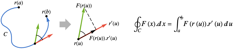
- Vector line integrals are used to compute the work done by a vector function along a curve in the direction of its tangent. Typical vector functions include a force field, electric field and fluid velocity field.
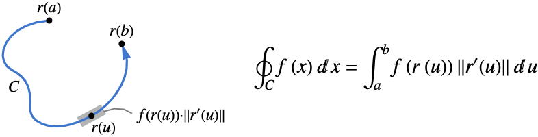
- The scalar line integral of the function f along a curve
 is given by:
 - … where
![TemplateBox[{{{r, ^, {(, ', )}}, (, u, )}}, Norm]](Files/NLineIntegrate.en/3.png "TemplateBox[{{{r, ^, {(, ', )}}, (, u, )}}, Norm]") is the measure of a parametric curve segment.
is the measure of a parametric curve segment. - The scalar line integral is independent of the parametrization and orientation of the curve. Any one-dimensional RegionQ object can be used as a curve.
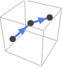
- The vector line integral of the function F along a curve
 is given by:
 - … where
).r^(')(u)") is projection of the vector function
is projection of the vector function  onto the tangent direction so only the component in the tangent direction gets integrated.
 - The vector line integral is independent of the parametrization of the curve, but it does depend on the orientation of the curve.
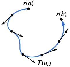
- The orientation for a curve is given by a tangent vector field
 over the curve.
 - For a parametric curve ParametricRegion[{r1[u],…,rn[u]},…], the tangent vector field
 is taken to be ∂ur[u].
 - Special curves in
 with their assumed tangent orientations include:
 -

Line[{p1,p2,…}] the orientation follows the points in the order they are given from p1 to p2 etc. 
HalfLine[{p1,p2}]
HalfLine[p,v]the orientation is from p1 to p2 or in the v direction 
InfiniteLine[{p1,p2}]
InfiniteLine[p,v]the orientation is from p1 to p2 or in the v direction 
Circle[p,r] the orientation is counterclockwise - Special curves in
 with their assumed tangent orientations include:
 -

Line[{p1,p2,…}] the orientation follows the points in the order they are given from p1 to p2 etc. 
HalfLine[{p1,p2}]
HalfLine[p,v]the orientation is from p1 to p2 or in the v direction 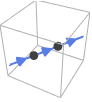
InfiniteLine[{p1,p2}]
InfiniteLine[p,v]the orientation is from p1 to p2 or in the v direction - Special curves in
 with their assumed tangent orientations include:
 -
Line[{p1,p2,…}] the orientation follows the points in the order they are given 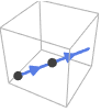
HalfLine[{p1,p2}]
HalfLine[p,v]the orientation is from p1 to p2 the orientation is given by v 
InfiniteLine[{p1,p2}]
InfiniteLine[p,v]the orientation is from p1 to p2 the orientation is given by v - The coordinates along the curve can be specified using VectorSymbol. »
- The following options can be given:
-
AccuracyGoal Infinity digits of absolute accuracy sought MaxPoints Automatic maximum total number of sample points MaxRecursion Automatic maximum number of recursive subdivisions Method Automatic method to use MinRecursion 0 minimum number of recursive subdivisions PrecisionGoal Automatic digits of precision sought WorkingPrecision MachinePrecision the precision used in internal computations
Examples
open all close allBasic Examples (6)
Line integral of a scalar field over a circle:
NLineIntegrate[2x, {x, y}∈Circle[{0, 0}, 1, {0, Pi / 2}]]Line integral of a vector field over a space curve:
NLineIntegrate[{x ^ 2 y z, 3x y, y ^ 2}, {x, y, z}∈ParametricRegion[{Cos[t], Sin[t], t}, {{t, 0, Pi / 2}}]]Line integral of a scalar field in two dimensions:
f = y ^ 2;Curve over which to integrate:
reg = ParametricRegion[{{t ^ (5 / 2), t}, 0 <= t <= 2}, {t}];A contour plot of ![]() and the curve:
and the curve:
Show[ContourPlot[f, {x, 0, 6}, {y, 0, 2}], ...]NLineIntegrate[f, {x, y}∈reg]Line integral of a vector field in two dimensions:
f = {x + 2y, x ^ 2};reg = Line[{{0, 0}, {2, 3 / 2}, {3, 0}}];The vector field and the integration path:
VectorPlot[f, {x, 0, 3}, {y, 0, 2}, ...]NLineIntegrate[f, {x, y}∈reg]Line integral of a vector field in three dimensions:
f = {z ^ 3, x ^ 3, y ^ 3};reg = Line[{{1, 1 / 2, 0}, {3, 2, 2}}];Show[VectorPlot3D[f, {x, 0, 4}, {y, 0, 2}, {z, 0, 2}, Rule[...]], ...]NLineIntegrate[f, {x, y, z}∈reg]Use VectorSymbol:
NLineIntegrate[VectorSymbol["x"].VectorSymbol["x"], VectorSymbol["x"]∈Line[{{0, 0}, {0, 1}}]]NLineIntegrate[x, x∈Line[{{0, 0}, {0, 1}}]]Scope (34)
Basic Uses (5)
Line integral of a scalar field:
f = Exp[x];NLineIntegrate[f, {x, y}∈Line[{{0, 0}, {2, 3}}]]Line integral of a vector field over a line segment:
NLineIntegrate[{x * y, x - y}, {x, y}∈Line[{{0, 0}, {1, 1}}]]Line integral of a vector field in three dimensions:
f = {x, x - y, z x ^ 2};NLineIntegrate[f, {x, y, z}∈ParametricRegion[{Sin[t], t, 2t}, {{t, 0, Pi}}]]LineIntegrate works with many special curves:
f = {x ^ 2 y, x};NLineIntegrate[f, {x, y}∈Annulus[{0, 0}, {1, 2}, {0, Pi / 4}]]//QuietLine integral over a parametric curve:
f = {Log[x], y};reg = ParametricRegion[{2t + 1, t ^ 2}, {{t, 0, 1}}];NLineIntegrate[f, {x, y}∈reg]Scalar Functions (11)
Line integral of a scalar field over a curve:
f = 2Abs[x - y] ^ (3 / 4);reg = ParametricRegion[{t, t ^ (3 / 2)}, {{t, 0, 8}}];Contour plot of ![]() and the curve:
and the curve:
Show[ContourPlot[f, {x, 0, 8}, {y, 0, 25}], ...]NLineIntegrate[f, {x, y}∈reg]Line integral of a scalar field over an arc of a circle:
f = 1 / (x + Sin[y] + 1) ^ 3;reg = Circle[{0, 0}, 1, {0, Pi / 2}];ContourPlot[f, {x, 0, 1}, {y, 0, 1}, Epilog -> reg, ImageSize -> Small]NLineIntegrate[f, {x, y}∈reg]Line integral of a scalar field over a parametric curve:
f = 1 / (x + 1) - y / 5;reg = ParametricRegion[{3 / 2t ^ 2, 4t}, {{t, -1, 1}}];Contour plot of the function and the curve:
Show[ContourPlot[f, {x, -1 / 2, 2}, {y, -4, 4}], ...]NLineIntegrate[f, {x, y}∈reg]Line integral of a scalar field over a circle:
f = Sin[1 / (x ^ 3 + y + 1)];reg = Circle[{2, 3}, 3];ContourPlot[f, {x, -1, 5}, {y, 0, 6}, Epilog -> reg, ImageSize -> Small]NLineIntegrate[f, {x, y}∈reg]Line integral of a scalar field over a space curve:
f = x + y - z;reg = ParametricRegion[{t ^ 3 / 3, Sqrt[2]t ^ 2 / 2, t}, {{t, 0, 1}}];NLineIntegrate[f, {x, y, z}∈reg]Line integral of a scalar field over the boundary of an annulus:
f = 1 / Exp[x + y + 5];reg = Annulus[{0, 0}, {1, 2}, {0, 3 / 4Pi}];Contour plot of the function and the curve:
ContourPlot[f, {x, -2, 4}, {y, -1, 5}, ...]NLineIntegrate[f, {x, y}∈reg]Line integral of a scalar field over a closed polygon:
f = Exp[Cos[Abs[x / 2 - y]]];reg = Line[{{0, 0}, {1, 2}, {0, 1}, {0, 0}}];Contour plot of the function and the curve:
ContourPlot[f, {x, 0, 1}, {y, 0, 2}, Epilog -> reg, AspectRatio -> Automatic]NLineIntegrate[f, {x, y}∈reg]Line integral of a scalar field over an elliptical path:
f = 2 x y;reg = Circle[{0, 0}, {1, 1 / Sqrt[2]}];Contour plot of the function and the curve:
ContourPlot[f, {x, -1, 1}, {y, -1, 1}, Epilog -> reg, ImageSize -> Small]NLineIntegrate[f, {x, y}∈reg]//QuietLine integral of a scalar field over a parametric curve:
f = x / 2 + Sin[y] ^ 2;reg = ParametricRegion[{6Cos[t] - Cos[6t], 6Sin[t] - Sin[6t]}, {{t, 0, 2Pi}}];Show[ContourPlot[f, {x, -10, 10}, {y, -10, 10}], RegionPlot[reg, BoundaryStyle -> Blue], ImageSize -> Small]NLineIntegrate[f, {x, y}∈reg, MaxRecursion -> 20]Line integral of a scalar field over a circle:
f = ArcTan[(y / x) ^ 2];reg = Circle[{0, 0}, 4];Contour plot of ![]() and the curve:
and the curve:
ContourPlot[f, {x, -4, 4}, {y, -4, 4}, Epilog -> reg, ImageSize -> Small]NLineIntegrate[f, {x, y}∈reg]Line integral of a scalar field over the boundary of a sector of a disk:
f = Cos[x - y];reg = Disk[{0, 0}, 3, {0, 3Pi / 4}];Contour plot of ![]() and the curve:
and the curve:
ContourPlot[f, {x, -3, 3}, {y, -1, 5}, ...]NLineIntegrate[f, {x, y}∈reg]Vector Functions (12)
Line integral of a vector field in three dimensions over a parametrized curve:
f = {2x, x, 1};reg = ParametricRegion[{Sin[t], Cos[t], t}, {{t, 0, 2Pi}}];Visualization of the vector field and the curve:
Show[VectorPlot3D[f, {x, -1, 1}, {y, -1, 1}, {z, 0, 7}, ...], ...]NLineIntegrate[f, {x, y, z}∈reg]Line integral of a vector field over a curve in two dimensions:
f = {Sin[x], y};reg = ParametricRegion[{t ^ 2, t ^ 3}, {{t, 0, 1}}];Show[VectorPlot[f, {x, 0, 1}, {y, 0, 1}, Rule[...]], ...]NLineIntegrate[f, {x, y}∈reg]Line integral of a vector field over a circular arc:
f = {x * (x ^ 2 + y ^ 2), y * (x ^ 2 + y ^ 2)};reg = Circle[{0, 0}, 1, {0, Pi / 2}];VectorPlot[f, {x, 0, 1}, {y, 0, 1}, ...]NLineIntegrate[f, {x, y}∈reg]//QuietLine integral of a vector field over a line segment:
f = {Sqrt[x ^ 2 + y ^ 2], Sqrt[Abs[x + y]]};reg = Line[{{0, 0}, {2, 2}, {4, 0}}];VectorPlot[f, {x, -1, 5}, {y, -1, 3}, ...]NLineIntegrate[f, {x, y}∈reg]Line integral of a vector field over a parametrized curve in three dimensions:
f = {x, x ^ 2 y ^ 2, 0};reg = ParametricRegion[{Cos[t] ^ 2, Cos[t]Sin[t], Sqrt[Cos[t](1 - Cos[t])]}, {{t, 0, 2Pi}}];Show[VectorPlot3D[f, {x, -1, 1}, {y, -1, 1}, {z, 0, 1}, Rule[...]], ...]NLineIntegrate[f, {x, y, z}∈reg]Line integral of a vector field over a curve:
f = {x + y, y + z, z + x};reg = ParametricRegion[{Sin[t] ^ 2 / Sqrt[2] + Cos[t] ^ 2, (1 - 1 / Sqrt[2])Cos[t]Sin[t], Sin[t] / Sqrt[2]}, {{t, 0, 2Pi}}];Show[VectorPlot3D[f, {x, 0, 1}, {y, -1, 1}, {z, -1, 1}, ...], ...]NLineIntegrate[f, {x, y, z}∈reg]Line integral of a vector field over an elliptical arc:
f = {x, Sin[x y ^ 2]};reg = Circle[{0, 0}, {2, 1}, {0, Pi}];VectorPlot[f, {x, -2, 2}, {y, -1 / 2, 3 / 2}, ...]NLineIntegrate[f, {x, y}∈reg]Line integral of a vector field over a parametric curve:
f = {x ^ 2, x ^ 2, Exp[y ^ 2 / 4]};reg = ParametricRegion[{(2 + Cos[3t])Cos[t], (2 + Cos[3t])Sin[t], Sin[3t]}, {{t, 0, 2Pi}}];Show[VectorPlot3D[f, {x, -3, 3}, {y, -3, 3}, {z, -1, 1}, ...], ...]NLineIntegrate[f, {x, y, z}∈reg]Line integral of a vector field over a parametric curve in three dimensions:
f = {(y - 1) ^ 2z, x ^ 2y, 2x y};reg = ParametricRegion[{Cos[t], Sin[t] / 2, Sin[t] / 2}, {{t, 0, Pi}}];Show[VectorPlot3D[f, {x, -1, 1}, {y, -1, 1}, {z, -1, 1}, Rule[...]], ...]NLineIntegrate[f, {x, y, z}∈reg]Line integral of a vector field over a parametrized curve:
f = {x ^ 2, 1 / 3, z ^ 2};reg = ParametricRegion[{2 / (1 + t ^ 2), 3t, 2t / (1 + t ^ 2)}, {{t, -10, 10}}];Show[VectorPlot3D[f, {x, 0, 2}, {y, -30, 30}, {z, -1, 1}, ...], ...]NLineIntegrate[f, {x, y, z}∈reg]Line integral of a vector field over an elliptical path:
f = {Sin[x ^ 4 y ^ 2], Sin[y]};reg = Circle[{0, 1}, {Sqrt[2], 1}];VectorPlot[f, {x, -2, 2}, {y, 0, 2}, ...]NLineIntegrate[f, {x, y}∈reg]Line integral of a vector field in higher dimensions:
f = {x y, x ^ 2t z, y t, z t};NLineIntegrate[f, {x, y, z, t}∈Line[{{0, 0, 0, 0}, {1, 2, 3, 4}}]]Special Curves (4)
Line integral over a circular arc:
f = Sqrt[x] * Abs[y] ^ (3 / 4);reg = Circle[{0, 0}, 4, {-Pi / 2, Pi / 2}];ContourPlot[f, {x, 0, 4}, {y, -4, 4}, ...]NLineIntegrate[f, {x, y}∈reg]Line integral of a vector field over the boundary of a circular sector of radius 1:
f = {Exp[Sin[3y]], y + x ^ 2};reg = Disk[{0, 0}, 1, {0, Pi / 2}];VectorPlot[f, {x, 0, 1}, {y, 0, 1}, ...]NLineIntegrate[f, {x, y}∈reg]f = {1 / (x + 2y) ^ 2, -1 / (x + y)};reg = Line[{{1, 0}, {0, 1}, {-1, 0}, {0, -1}, {1, 0}}];VectorPlot[f, {x, -1, 1}, {y, -1, 1}, ...]NLineIntegrate[f, {x, y}∈reg]//QuietLine integral over the boundary of an annulus:
f = {-2y, x};reg = Annulus[{0, 0}, {1, 2}, {0, Pi / 4}];VectorPlot[f, {x, 0, 2}, {y, 0, 2}, ...]NLineIntegrate[f, {x, y}∈reg, AccuracyGoal -> 5]Parametric Curves (2)
Line integral of a vector field over a spiral in three dimensions:
f = {y - z, z - x, x - y};reg = ParametricRegion[{ Cos[t], Sin[t], t}, {{t, 0, 2Pi}}];Show[VectorPlot3D[f, {x, -1, 1}, {y, -1, 1}, {z, 0, 2Pi}, ...], ...]NLineIntegrate[f, {x, y, z}∈reg]Line integral of a scalar field over a parametric curve:
NLineIntegrate[Exp[-x], {x, y}∈ParametricRegion[{2t, 3t}, {{t, 0, Infinity}}]]Options (8)
AccuracyGoal (1)
The option AccuracyGoal sets the number of digits of accuracy:
exact = LineIntegrate[{1, x ^ 2}, {x, y}∈Circle[]]NLineIntegrate[{1, x ^ 2}, {x, y}∈Circle[], AccuracyGoal -> 15] - exactThe result with default settings only sets a PrecisionGoal:
NLineIntegrate[{1, x ^ 2}, {x, y}∈Circle[]] - exactMaxPoints (1)
MaxRecursion (1)
The option MaxRecursion specifies the maximum number of recursive steps:
reg = ParametricRegion[{Sin[t], 1}, {{t, 0, Pi}}];NLineIntegrate[{1 / Sqrt[x], x}, {x, y}∈reg]
Increasing the number of recursions:
NLineIntegrate[{1 / Sqrt[x], x}, {x, y}∈reg, MaxRecursion -> 20]LineIntegrate[{1 / Sqrt[x], x}, {x, y}∈reg]Method (1)
The option Method can take the same values as in NIntegrate. For example:
NLineIntegrate[{-Sin[y] ^ 3, x ^ 2}, {x, y}∈Circle[], Method -> "TrapezoidalRule", WorkingPrecision -> 15]NLineIntegrate[{-Sin[y] ^ 3, x ^ 2}, {x, y}∈Circle[], Method -> "NewtonCotesRule", WorkingPrecision -> 15]NLineIntegrate[{-Sin[y] ^ 3, x ^ 2}, {x, y}∈Circle[], Method -> "ClenshawCurtisRule", WorkingPrecision -> 15]NLineIntegrate[{-Sin[y] ^ 3, x ^ 2}, {x, y}∈Circle[], WorkingPrecision -> 15]Compare to the truncated exact result:
LineIntegrate[{-Sin[y] ^ 3, x ^ 2}, {x, y}∈Circle[]]%//N[#, 15]&MinRecursion (1)
The option MinRecursion forces a minimum number of subdivisions:
NLineIntegrate[Exp[-100(x ^ 2 + y ^ 2)], {x, y}∈Line[{{-60, -60}, {60, 60}}]]NLineIntegrate[Exp[-100(x ^ 2 + y ^ 2)], {x, y}∈Line[{{-60, -60}, {60, 60}}], MinRecursion -> 5]LineIntegrate[Exp[-100(x ^ 2 + y ^ 2)], {x, y}∈Line[{{-60, -60}, {60, 60}}]]N[%]PrecisionGoal (1)
The option PrecisionGoal sets the relative tolerance in the integration:
exact = LineIntegrate[{Exp[-y ^ 2], Sin[x]}, {x, y}∈Circle[{0, 0}, {1, 2}]]NLineIntegrate[{Exp[-y ^ 2], Sin[x]}, {x, y}∈Circle[{0, 0}, {1, 2}], PrecisionGoal -> 20, MaxRecursion -> 20, WorkingPrecision -> 20] - exactNLineIntegrate[{Exp[-y ^ 2], Sin[x]}, {x, y}∈Circle[{0, 0}, {1, 2}]] - exactWorkingPrecision (2)
If a WorkingPrecision is specified, the computation is done at that working precision:
NLineIntegrate[1, {x, y}∈Circle[]]NLineIntegrate[1, {x, y}∈Circle[], WorkingPrecision -> 16]The result has finite precision if the integrand has a finite precision:
NLineIntegrate[{-y, 0.567x}, {x, y}∈Line[{{0, 0}, {2, 4}}]]Applications (27)
College Calculus (10)
Line integral of a function ![]() over a line segment:
over a line segment:
f = Exp[x] y ^ 2 z ^ (3 / 2);reg = Line[{{-1, 3, 1}, {1, 7, 3}}];NLineIntegrate[f, {x, y, z}∈reg]Line integral of a vector field over a curve:
f = {x Sin[y], y Cos[z], z Sin[x]};reg = ParametricRegion[{Cos[t], Sin[t] ^ 2, -Cos[t]}, {{t, 0, Pi}}];NLineIntegrate[f, {x, y, z}∈reg]Mass of a thin circular wire of radius 1 with linear density ![]() :
:
ρ = BesselJ[1, x ^ 2 / 2] * y ^ 2;reg = Circle[{0, 0}, 1];NLineIntegrate[ρ, {x, y}∈reg]Work done by the force field ![]() on a particle that moves along a line segment:
on a particle that moves along a line segment:
f = {x - y ^ 3, y - z ^ 3, z - x ^ 3};reg = Line[{{0, 0, 0}, {1, 2, 3}}];NLineIntegrate[f, {x, y, z}∈reg]Line integral of a vector field along a path:
f = {Cos[x], Sin[y]};reg = Line[{{0, 0}, {3, 0}, {3, 3}, {0, 3}, {0, 0}}];NLineIntegrate[f, {x, y}∈reg]Line integral of a vector field along a curve:
f = {ArcTan[x ^ 2], y ^ 2};reg = ParametricRegion[{t, t ^ 2}, {{t, 0, 1}}];NLineIntegrate[f, {x, y}∈reg]Work done by the force ![]() as a particle moves along the curve
as a particle moves along the curve ![]() :
:
f = {x ^ 2, y};reg = ParametricRegion[{t - Sin[t], 1 - Cos[t]}, {{t, 0, 2Pi}}];NLineIntegrate[f, {x, y}∈reg]Line integral of a vector field along the unit circle centered at the origin:
f = {x + y, x ^ 2};NLineIntegrate[f, {x, y}∈Circle[]]Line integral of a vector field along a circle of radius 2 centered at the origin:
f = {x ^ 2 / (x ^ 2 + y ^ 2), (y ^ 2 - x ^ 2) / (x ^ 2 + y ^ 2)};NLineIntegrate[f, {x, y}∈Circle[{0, 0}, 2]]//QuietNumerical value of the line integral of a vector field over a path:
f = {Exp[Sin[x ^ 2]], Exp[Sqrt[x ^ 2 + y ^ 2]]};reg = ParametricRegion[{Sin[t ^ 2], Cos[t] ^ 3}, {{t, 0, 2Pi}}];NLineIntegrate[f, {x, y}∈reg, WorkingPrecision -> 16]Lengths (3)
NLineIntegrate[1, {x, y}∈Circle[]]Perimeter of a cardioid using a line integral:
reg = ParametricRegion[{(2Cos[t] - Cos[2t]), (2Sin[t] - Sin[2t])}, {{t, 0, 2Pi}}];RegionPlot[reg, ImageSize -> Small]NLineIntegrate[1, {x, y}∈reg]The length can also be calculated with RegionMeasure:
RegionMeasure[reg]reg = ParametricRegion[{Cos[t] ^ 3, Sin[t] ^ 3}, {{t, 0, 2Pi}}];RegionPlot[reg, ImageSize -> Small]NLineIntegrate[1, {x, y}∈reg]Areas (5)
Area of an ellipse with semiaxes of length 2 and 3, calculated using a line integral:
NLineIntegrate[{-y / 2, x / 2}, {x, y}∈Circle[{0, 0}, {2, 3}]]Area of the right-hand loop of the lemniscate ![]() computed using a line integral:
computed using a line integral:
f = {-y / 2, x / 2};reg = ParametricRegion[{Sqrt[Cos[2ϕ]]Cos[ϕ], Sqrt[Cos[2ϕ]]Sin[ϕ]}, {{ϕ, -Pi / 4, Pi / 4}}];Show[VectorPlot[f, {x, 0, 1}, {y, -1 / 2, 1 / 2}, ...], ...]NLineIntegrate[f, {x, y}∈reg]Area of the epicycloid of parameters ![]() and
and ![]() :
:
R = 2;r = 1 / 2;reg = ParametricRegion[{(R + r)Cos[t] - r Cos[(R + r) / r * t], (R + r)Sin[t] - r Sin[(R + r) / r * t]}, {{t, 0, 2Pi}}];Show[VectorPlot[{-y / 2, x / 2}, {x, -3, 3}, {y, -3, 3}, ...], ...]NLineIntegrate[{-y / 2, x / 2}, {x, y}∈reg]Area of the cardioid using a line integral:
reg = ParametricRegion[{(2Cos[t] - Cos[2t]), (2Sin[t] - Sin[2t])}, {{t, 0, 2Pi}}];RegionPlot[reg, ImageSize -> Small]NLineIntegrate[{-y / 2, x / 2}, {x, y}∈reg]Area of an astroid using a line integral:
reg = ParametricRegion[{Cos[t] ^ 3, Sin[t] ^ 3}, {{t, 0, 2Pi}}];RegionPlot[reg, ImageSize -> Small]NLineIntegrate[{-y / 2, x / 2}, {x, y}∈reg]Work by a Force (4)
Work done by a force ![]() force as an object is moved on a straight line:
force as an object is moved on a straight line:
f = {0, 0, -1};NLineIntegrate[f, {x, y, z}∈Line[{{0, 0, 0}, {1, 2, 3}}]]Work done by the electric force as a charged particle of charge ![]() is moved from {1,1,0} to {2,2,0} in the electric field of a charged infinite wire of charge density
is moved from {1,1,0} to {2,2,0} in the electric field of a charged infinite wire of charge density ![]() :
:
Subscript[ϵ, 0] = 8.854 * 10 ^ -12;q = 10 ^ -6;λ = 10 ^ -5;f = {(λ * q * x/2Pi Subscript[ϵ, 0](x ^ 2 + y ^ 2)), (λ * q * y/2Pi Subscript[ϵ, 0](x ^ 2 + y ^ 2)), 0};NLineIntegrate[f, {x, y, z}∈Line[{{1, 1, 0}, {2, 2, 0}}]]Work done by an elastic force directed toward the origin as a quarter of an ellipse is traced:
f = {-2x, -2y};reg = Circle[{0, 0}, {1, 2}, {0, Pi / 2}];NLineIntegrate[f, {x, y}∈reg]Work of the electric force as a charge ![]() is moved along the
is moved along the ![]() axis from
axis from ![]() to infinity in the electric field of a charge
to infinity in the electric field of a charge ![]() :
:
Subscript[ϵ, 0] = 8.854 * 10 ^ -12;Q = 2. * 10 ^ -5;q = 10 ^ -5;Subscript[x, 0] = 1;f = {(Q * q * x/4π Subscript[ϵ, 0](x ^ 2 + y ^ 2 + z ^ 2) ^ (3 / 2)), (Q * q * y/4π Subscript[ϵ, 0](x ^ 2 + y ^ 2 + z ^ 2) ^ (3 / 2)), (Q * q * z/4π Subscript[ϵ, 0](x ^ 2 + y ^ 2 + z ^ 2) ^ (3 / 2))};reg = ParametricRegion[{Subscript[x, 0] + t, 0, 0}, {{t, 0, Infinity}}];NLineIntegrate[f, {x, y, z}∈reg]Centroids (2)
Mass of a closed semicircular wire of radius 2 and unit linear density:
reg = Disk[{0, 0}, 2, {0, Pi}];m = NLineIntegrate[1, {x, y}∈reg]![]() coordinate of the center of mass:
coordinate of the center of mass:
(1 / m) * NLineIntegrate[x, {x, y}∈reg, AccuracyGoal -> 5]![]() coordinate of the center of mass:
coordinate of the center of mass:
(1 / m) * NLineIntegrate[y, {x, y}∈reg, AccuracyGoal -> 5]Moments of inertia of a helix-shaped wire of unit linear density:
reg = ParametricRegion[{Cos[t], Sin[t], t / 10}, {{t, 0, 6Pi}}];ParametricPlot3D[{Cos[t], Sin[t], t / 10}, {t, 0, 6Pi}, ImageSize -> Small]NLineIntegrate[(y ^ 2 + z ^ 2), {x, y, z}∈reg]NLineIntegrate[(x ^ 2 + z ^ 2), {x, y, z}∈reg]NLineIntegrate[(x ^ 2 + y ^ 2), {x, y, z}∈reg]Classical Theorems (3)
A vector field is conservative if its line integral depends only on the values at the endpoints, not on the path:
f = {3 x^2 y, x^3};The field ![]() is the gradient of a scalar function
is the gradient of a scalar function ![]() :
:
g = x ^ 3 y;f == Grad[g, {x, y}]All gradients of scalar fields are conservative. For example, the line integral of ![]() over the curve is:
over the curve is:
reg = ParametricRegion[{t ^ 2, Exp[t]}, {{t, 0, 1}}];NLineIntegrate[f, {x, y}∈reg]This is the same as the difference of the values of ![]() at the endpoints of the curve:
at the endpoints of the curve:
(g /. {x -> t ^ 2, y -> Exp[t]} /. t -> 1) - (g /. {x -> t ^ 2, y -> Exp[t]} /. t -> 0)//NGreen's theorem. The line integral of the vector field ![]() over a closed curve is:
over a closed curve is:
f = {x ^ 4, x * y ^ 2 + 1};NLineIntegrate[f, {x, y}∈Line[{{0, 0}, {1, 0}, {0, 1}, {0, 0}}]]This can be related to a surface integral of ![]() over the region enclosed by the curve, where
over the region enclosed by the curve, where ![]() is defined as:
is defined as:
g = D[f[[2]], x] - D[f[[1]], y];NIntegrate[g, {x, y}∈Triangle[{{0, 0}, {1, 0}, {0, 1}}]]Stokes's theorem. The line integral of a vector field ![]() along a closed line in three dimensions is:
along a closed line in three dimensions is:
f = {-y + x y ^ 2, x, z};reg = ParametricRegion[{Cos[t], Sin[t], 0}, {{t, 0, 2Pi}}];NLineIntegrate[f, {x, y, z}∈reg]This is equal to the surface integral of the Curl of ![]() on any surface having the curve as its boundary:
on any surface having the curve as its boundary:
reg2 = ParametricRegion[{Cos[t]Cos[p], Cos[t]Sin[p], Sin[t]}, {{p, 0, 2Pi}, {t, 0, Pi / 2}}];NSurfaceIntegrate[Curl[f, {x, y, z}], {x, y, z}∈reg2]The surface integral across a different surface with the same boundary is the same:
NSurfaceIntegrate[Curl[f, {x, y, z}], {x, y, z}∈ParametricRegion[{r Cos[t], r Sin[t], 0}, {{r, 0, 1}, {t, 0, 2Pi}}]]Properties & Relations (5)
Apply N[LineIntegrate[…]] to obtain a numerical solution if the symbolic calculation fails:
f = Sin[x + y + z];reg = ParametricRegion[{t ^ 2, t ^ 3, t ^ 4}, {{t, 0, 1}}];LineIntegrate[f, {x, y, z}∈reg]N[LineIntegrate[f, {x, y, z}∈reg]]NLineIntegrate[f, {x, y, z}∈reg]Find the center of mass of a triangular wire of unit linear density:
reg = Line[{{0, 0}, {1, 0}, {1, 1}, {0, 0}}];RegionPlot[reg, ImageSize -> Small]m = NLineIntegrate[1, {x, y}∈reg]Find the ![]() component of the center of mass:
component of the center of mass:
1 / m * NLineIntegrate[x, {x, y}∈reg]1 / m * NLineIntegrate[y, {x, y}∈reg]//QuietThe center of mass can also be obtained using RegionCentroid:
RegionCentroid[reg]//NFind the moment of inertia around the ![]() axis of a circular wire of unit linear density centered at the origin in the
axis of a circular wire of unit linear density centered at the origin in the ![]() -
-![]() plane:
plane:
reg = ParametricRegion[{Cos[t], Sin[t], 0}, {{t, 0, 2Pi}}];NLineIntegrate[(x ^ 2 + y ^ 2), {x, y, z}∈reg]The answer can also be computed with MomentOfInertia:
MomentOfInertia[reg, {0, 0, 0}, {0, 0, 1}]//NFind the length of an epicycloid:
reg = ParametricRegion[{6 Cos[t] - Cos[6 t], 6 Sin[t] - Sin[6 t]}, {{t, 0, 2Pi}}];RegionPlot[reg, ImageSize -> Small]NLineIntegrate[1, {x, y}∈reg]//QuietThe same answer can be obtained using ArcLength:
ArcLength[{6 Cos[t] - Cos[6 t], 6 Sin[t] - Sin[6 t]}, {t, 0, 2Pi}]reg = Circle[{0, 0}, {1 / Sqrt[2], 1 / Sqrt[3]}];NLineIntegrate[{-y / 2, x / 2}, {x, y}∈reg]The result can be obtained using RegionMeasure:
RegionMeasure[Disk[{0, 0}, {1 / Sqrt[2], 1 / Sqrt[3]}]]Neat Examples (2)
reg = ParametricRegion[{t, Cosh[t]}, {{t, -1, 1}}];ParametricPlot[{t, Cosh[t]}, {t, -1, 1}, ImageSize -> Small]NLineIntegrate[1, {x, y}∈reg]Integral of a vector field over a Clelia curve:
f = {x ^ 2 + y, y ^ 2 + z, z ^ 2 + x};reg = ParametricRegion[{Cos[t]Cos[3t], Cos[t]Sin[3t], Sin[t]}, {{t, 0, 2Pi}}];Show[VectorPlot3D[f, {x, -1, 1}, {y, -1, 1}, {z, -1, 1}, Rule[...]], ...]NLineIntegrate[f, {x, y, z}∈reg]Text
Wolfram Research (2024), NLineIntegrate, Wolfram Language function, https://reference.wolfram.com/language/ref/NLineIntegrate.html (updated 2025).
CMS
Wolfram Language. 2024. "NLineIntegrate." Wolfram Language & System Documentation Center. Wolfram Research. Last Modified 2025. https://reference.wolfram.com/language/ref/NLineIntegrate.html.
APA
Wolfram Language. (2024). NLineIntegrate. Wolfram Language & System Documentation Center. Retrieved from https://reference.wolfram.com/language/ref/NLineIntegrate.html