

RayleighDistribution
尺度母数 σ のレイリー(Rayleigh)分布を表す.
詳細
- レイリー分布における値
 の確率密度は,
 では
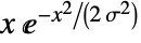 に比例し,
 では0である. »
- RayleighDistributionでは,σ は正の実数でよい.
- RayleighDistributionでは,σ は任意の単位次元の数量でよい. »
- RayleighDistributionは,Mean,CDF,RandomVariate等の関数で使うことができる. »
予備知識
- RayleighDistribution[σ]分布は,区間
 上でサポートされ,確率密度関数(PDF)の全体的な動作を決定する正の実数 σ(「尺度母数」と呼ばれる)でパラメータ化された連続統計分布を表す.一般に,レイリー分布のPDFは,単一の「峰」(大域的最大値)を持つ単峰性であるが,その全体的な形(高さ,広がり,最大値の水平位置)は σ の値によって決まる.加えて,PDFの裾部は,PDFが
 の大きい値について代数的というよりむしろ指数的に減少するという意味で「薄い」(この動作は,分布のSurvivalFunctionを分析することで数量的に厳密にできる).
- レイリー分布は,そ1880年代の初めに,その名前が取られたLord Rayleighによって,音響学のある種の問題を解くためのツールとして導き出された.数学では,レイリー分布は,変数
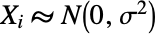 がすべて独立同分布に従う標準変量である場合は常に,
 上の原点から点
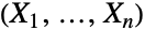 までの距離の確率分布である.さらに,レイリー分布は,二次元ランダムウォークや電気真空デバイスの製造欠陥等を含むさまざまな現象をモデル化することが証明されており,ポアソ過程が生成した空間形状における個とその最近傍の距離の分布でもある.
- RandomVariateを使って,レイリー分布から,1つあるいは複数の機械精度あるいは任意精度(後者はWorkingPrecisionオプションを介す)の擬似乱数変量を得ることができる.Distributed[x,RayleighDistribution[σ]](より簡略な表記では xRayleighDistribution[σ])を使って,確率変数 x がレイリー分布に従って分布していると宣言することができる.このような宣言は,Probability,NProbability,Expectation,NExpectation等の関数で使うことができる.
- 確率密度関数および累積分布関数は,PDF[RayleighDistribution[σ],x]およびCDF[RayleighDistribution[σ],x]を使って得られることがある.平均,中央値,分散,原点の周りのモーメント,中心モーメントは,それぞれMean,Median,Variance,Moment,CentralMomentを使って計算することができる.
- DistributionFitTestを使って,与えられたデータ集合がレイリー分布と一致するかどうかを検定することが,EstimatedDistributionを使って与えられたデータからパラメトリックレイリー分布を推定することが,FindDistributionParametersを使ってデータをレイリー分布にフィットすることができる.ProbabilityPlotを使って記号レイリー分布のCDFに対する与えられたデータのCDFのプロットを生成することが,QuantilePlotを使って記号レイリー分布の変位値に対する与えられたデータの変位値のプロットを生成することができる.
- TransformedDistributionを使って変換されたレイリー分布を表すことが,CensoredDistributionを使って上限値と下限値の間で切り取られた値の分布を表すことが,TruncatedDistributionを使って上限値と下限値の間で切断された値の分布を表すことができる.CopulaDistributionを使ってレイリー分布を含む高次元分布を構築することが,ProductDistributionを使ってレイリー分布を含む独立成分分布の結合分布を計算することができる.
- RayleighDistributionは数多くの他の分布と関連がある.RayleighDistributionは,RayleighDistribution[1]とChiDistribution[2]のPDFが等しく,RayleighDistribution[1]とChiSquareDistribution[2]のCDFが等しいという意味で,ChiDistributionおよびChiSquareDistributionと関連がある.RayleighDistributionは,RayleighDistribution[σ]のPDFがRiceDistribution[0,σ],GammaDistribution[1,σ
 , 2, 0],WeibullDistribution[2,σ
 ]のPDFと等しいことから,RiceDistribution,GammaDistribution,WeibullDistributionの特殊ケースとして実現することができ,さらに,ExponentialDistributionおよびBeniniDistributionの変換としても実現することができる.RayleighDistributionは,NormalDistribution,BinormalDistribution,LaplaceDistribution,SuzukiDistribution,LogNormalDistribution,KDistributionとも関連している.
例題
すべて開く すべて閉じる例 (4)
Plot[Table[PDF[RayleighDistribution[σ], x], {σ, {.5, 1, 2}}]//Evaluate, {x, 0, 6}, Filling -> Axis, PlotRange -> All]PDF[RayleighDistribution[σ], x]Plot[Table[CDF[RayleighDistribution[σ], x], {σ, {.5, 1, 2}}]//Evaluate, {x, 0, 6}, Filling -> Axis, PlotRange -> All]CDF[RayleighDistribution[σ], x]Mean[RayleighDistribution[σ]]N[%]Variance[RayleighDistribution[σ]]N[%]Median[RayleighDistribution[σ]]N[%]スコープ (7)
data = RandomVariate[RayleighDistribution[2], 10 ^ 4];Show[
Histogram[data, 20, "PDF"],
Plot[PDF[RayleighDistribution[2], x], {x, 0, 8}, PlotStyle -> Thick]]sample = RandomVariate[RayleighDistribution[3], 10 ^ 3];edist = EstimatedDistribution[sample, RayleighDistribution[σ]]サンプルの密度ヒストグラムを推定分布の確率密度関数と比較する:
Show[Histogram[sample, Automatic, "PDF"], Plot[PDF[edist, x], {x, 0, 10}, PlotStyle -> Thick]]Skewness[RayleighDistribution[σ]]N[%]Kurtosis[RayleighDistribution[σ]]N[%]FormulaGrid[list_, type_] := Grid[...]FormulaGrid[Table[Moment[RayleighDistribution[σ], k], {k, 5}], M]Moment[RayleighDistribution[σ], r]FormulaGrid[Table[CentralMoment[RayleighDistribution[σ], k]//Factor, {k, 5}], CM]FormulaGrid[Table[FactorialMoment[RayleighDistribution[σ], k]//Factor, {k, 5}], FM]FormulaGrid[Table[Cumulant[RayleighDistribution[σ], k]//Factor, {k, 5}], C]Plot[Table[HazardFunction[RayleighDistribution[σ], x], {σ, {0.5, 0.75, 1}}]//Evaluate, {x, 0, 4}, Filling -> Axis]HazardFunction[RayleighDistribution[σ], x]Plot[Table[Quantile[RayleighDistribution[σ], q], {σ, {0.5, 1, 2}}]//Evaluate, {q, 0, 1}, Filling -> Axis]Quantile[RayleighDistribution[σ], q]母数でQuantityを一貫して使うとQuantityDistributionが与えられる:
serviceTime𝒟 = RayleighDistribution[Quantity[10, "Years"]]Mean[serviceTime𝒟]//Nアプリケーション (7)
Table[Arrow[{{0, 0}, RandomVariate[NormalDistribution[], 2]}], {100}]//Graphicsvectors = RandomVariate[NormalDistribution[], {10^4, 2}];Show[Histogram[Apply[ArcTan, vectors, {1}], Automatic, "PDF"], Plot[PDF[UniformDistribution[{-π, π}], x], {x, -π, π}, PlotStyle -> Thick]]Show[Histogram[Map[Norm, vectors], 25, "PDF"], Plot[PDF[RayleighDistribution[1], x], {x, 0, 5}, PlotStyle -> Thick]]TransformedDistribution[Norm[{u, v}], {uNormalDistribution[], vNormalDistribution[]}]ある製品の故障までの時間は母数 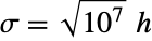 でレイリー分布に従っている.使用開始から4000時間,4500時間,5000時間後の製品の信頼性はどうであろうか.信頼性は生存確率としても知られる:
time𝒟 = RayleighDistribution[Quantity[Sqrt[10^7], "Hours"]]Table[SurvivalFunction[time𝒟, t], {t, Quantity[{4000., 4500., 5000.}, "Hours"]}]あるデバイスの寿命がレイリー分布に従うものとして,そのデバイスの信頼性を求める:
SurvivalFunction[RayleighDistribution[σ], t]HazardFunction[RayleighDistribution[σ], t]rs = SurvivalFunction[RayleighDistribution[σ1], t]SurvivalFunction[RayleighDistribution[σ2], t]//PiecewiseExpandrp = 1 - (1 - SurvivalFunction[RayleighDistribution[σ1], t])(1 - SurvivalFunction[RayleighDistribution[σ2], t])//PiecewiseExpand

Block[{σ1 = 2, σ2 = 3}, Plot[{Legended[rs, "in series"], Legended[rp, "in parallel"]}, {t, 0, 10}]]ベクトルには正規分布に従う2つの構成要素がある.ベクトルの長さの分布を求める:
𝒟 = TransformedDistribution[Norm[{u, v}], {uNormalDistribution[], vNormalDistribution[]}]Plot[PDF[𝒟, x], {x, 0, 5}, Filling -> Axis]Mean[𝒟]30個のベクトルサンプルの可能な長さのシミュレーションを行う:
ListPlot[{RandomVariate[𝒟, 30], {{0, Mean[𝒟]}, {30, Mean[𝒟]}}}, Joined -> {False, True}, Filling -> Axis, AxesOrigin -> {0, 0}]RayleighDistributionを使って風速を近似することができる:
wind = WeatherData["Copenhagen", "WindSpeed", {{2006, 1, 1}, {2009, 12, 31}, "Day"}]windEstimate = EstimatedDistribution[wind, RayleighDistribution[σ]]Show[Histogram[wind, Automatic, "PDF", AxesLabel -> Automatic], Plot[PDF[windEstimate, Quantity[x, "km/h"]], {x, 0, 35}, PlotStyle -> Thick]]Probability[x > Quantity[30, "Kilometers"/"Hours"], xwindEstimate]Mean[windEstimate]ListPlot[{RandomVariate[windEstimate, 30], {{0, Mean[windEstimate]}, {30, Mean[windEstimate]}}}, Joined -> {False, True}, Filling -> Axis, AxesOrigin -> {0, 0}, AxesLabel -> {"days", Automatic}]ある場所における上位1/3の高さの波の平均を  とする.この場所における波の高さはRayleighDistributionでモデル化することができる:
𝒟 = RayleighDistribution[H / 2];SurvivalFunction[𝒟, x]
Probability[x > H, x𝒟]N[%]Mean[𝒟]N[%] メートルであると仮定して,波の高さのシミュレーションを行う:
ListPlot[RandomVariate[𝒟 /. H -> Quantity[12, "m"], 100], Joined -> True, AxesLabel -> Automatic]フェージングチャネル理論では,RayleighDistributionを使って線が直接見えない場合のフェージング振幅をモデル化する.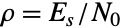 で瞬間的な信号対ノイズ比の分布を求める.
 は記号あたりのエネルギー,
 はホワイトノイズのスペクトル密度である:
SNRdist = TransformedDistribution[ρ u ^ 2, uRayleighDistribution[σ]]; がExponentialDistributionであることを示す:
PDF[SNRdist, x]//Refine[#, ρ > 0]&PDF[ExponentialDistribution[1 / (2 ρ σ ^ 2)], x]FullSimplify[% - %%, x > 0]MomentGeneratingFunction[SNRdist, t]Mean[SNRdist](1 - Mean[SNRdist] t) ^ -1 == MomentGeneratingFunction[SNRdist, t]//FullSimplifyAF[dist_] := Variance[dist] / (Mean[dist]) ^ 2AF[SNRdist]特性と関係 (14)
レイリー分布は正の因子によるスケーリングの下では閉じている:
TransformedDistribution[k * u, uRayleighDistribution[σ]]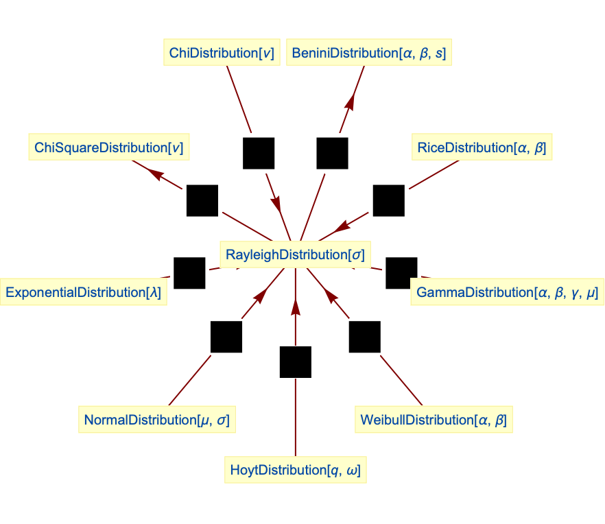
 のRayleighDistributionはChiDistributionの特殊なケースである:
PDF[RayleighDistribution[1], x]PDF[ChiDistribution[2], x]Simplify[% - %%] のRayleighDistributionの平方はChiSquareDistributionの特殊なケースである:
CDF[RayleighDistribution[1], Sqrt[x]]CDF[ChiSquareDistribution[2], x]Simplify[% - %%, x > 0]レイリー分布はRiceDistributionの特殊ケースである:
PDF[RayleighDistribution[β], x]PDF[RiceDistribution[0, β], x]% - %%RayleighDistributionはGammaDistributionの特殊ケースである:
PDF[GammaDistribution[1, σSqrt[2], 2, 0], x]PDF[RayleighDistribution[σ], x]% - %%BeniniDistributionはレイリー分布を変換したものである:
𝒟 = TransformedDistribution[Exp[u], uRayleighDistribution[σ]];PDF[𝒟, x]PDF[BeniniDistribution[0, 1 / (2σ ^ 2), 1], x]FullSimplify[% - %%, x > 1]TransformedDistribution[Norm[{u, v}], {uNormalDistribution[], vNormalDistribution[]}]NormalDistributionとレイリー分布の母数混合分布はLaplaceDistributionである:
𝒟 = ParameterMixtureDistribution[NormalDistribution[μ, σ], σRayleighDistribution[ν]]レイリー分布はBinormalDistributionに関連している:
𝒟 = TransformedDistribution[Norm[{u, v}], {u, v}BinormalDistribution[{0, 0}, {σ, σ}, 0]];Block[{σ = 2}, Show[Histogram[RandomVariate[𝒟, 10 ^ 4], 20, "PDF"], Plot[PDF[RayleighDistribution[σ], x], {x, 0, 8}, PlotStyle -> Thick]]]レイリー分布はWeibullDistributionの特殊ケースである:
PDF[WeibullDistribution[2, Sqrt[2]σ], x]PDF[RayleighDistribution[σ], x]% - %%レイリー分布はExponentialDistributionを変換したものとして求めることができる:
TransformedDistribution[Sqrt[2 u], uExponentialDistribution[1 / σ ^ 2], Assumptions -> σ > 0]PDF[RayleighDistribution[σ], x] === PDF[%, x]SuzukiDistributionはLogNormalDistributionとレイリー分布から得ることができる:
𝒟 = TransformedDistribution[u z, {uRayleighDistribution[1], zLogNormalDistribution[μ, ν]}];Block[{μ = -1, ν = 1 / 5}, Show[Histogram[RandomVariate[𝒟, 10 ^ 4], 25, "PDF"], Plot[PDF[SuzukiDistribution[μ, ν], x], {x, 0, 2}, PlotStyle -> Thick]]]KDistributionはRayleighDistributionとGammaDistributionの母数混合として表すことができる:
𝒟 = ParameterMixtureDistribution[RayleighDistribution[Sqrt[σ]], σGammaDistribution[α, β / (2α)]]考えられる問題 (2)
RayleighDistributionは,σ が正の実数ではないときは定義されない:
Mean[RayleighDistribution[-1]]
Mean[RayleighDistribution[σ]] /. {σ -> 3 + I}おもしろい例題 (2)
Table[Arrow[{{0, 0}, RandomVariate[NormalDistribution[], 2]}], {100}]//Graphics結果の二変量分布はそのラジアル方向でRayleighDistributionに従う:
RevolutionPlot3D[(1/2π)PDF[RayleighDistribution[1], r], {r, 0, 4}, PlotStyle -> Opacity[0.8], PlotPoints -> 35, Mesh -> None]Integrate[(1/2π)PDF[RayleighDistribution[1], r], {r, 0, ∞}, {θ, 0, 2π}]RevolutionPlot3D[CDF[RayleighDistribution[1], r], {r, 0, 4}, PlotStyle -> Opacity[0.8], PlotPoints -> 35, Mesh -> None]累積分布関数の等高線を持つ σ のさまざまな値についての確率密度関数:
dist = RayleighDistribution[σ];cdf = Function[{x, σ}, Evaluate[CDF[dist, x]]];
ql = {0.025, 0.10, 0.25, 0.5, 0.75, 0.90, 0.975};
cl = Table[ColorData["Rainbow"][q], {q, Join[{0.0}, ql]}];Legended[Plot3D[PDF[dist, x], {x, 0, 1}, {σ, 0.1, 1}, PlotTheme -> "Marketing", MeshFunctions -> {cdf}, Mesh -> {ql}, MeshStyle -> GrayLevel[0.8], MeshShading -> cl, AxesLabel -> Automatic, BaseStyle -> Opacity[0.9], ImageSize -> 400, PlotPoints -> 50, PlotRange -> All], BarLegend["Rainbow", ql, LegendLabel -> "prob"]]テキスト
Wolfram Research (2007), RayleighDistribution, Wolfram言語関数, https://reference.wolfram.com/language/ref/RayleighDistribution.html (2016年に更新).
CMS
Wolfram Language. 2007. "RayleighDistribution." Wolfram Language & System Documentation Center. Wolfram Research. Last Modified 2016. https://reference.wolfram.com/language/ref/RayleighDistribution.html.
APA
Wolfram Language. (2007). RayleighDistribution. Wolfram Language & System Documentation Center. Retrieved from https://reference.wolfram.com/language/ref/RayleighDistribution.html