


AudioLocalMeasurements
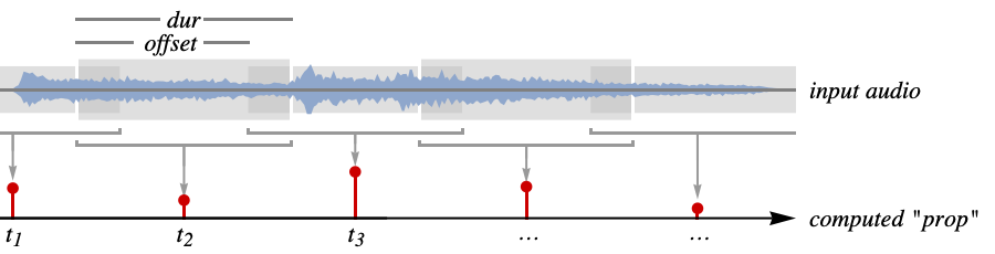
AudioLocalMeasurements[audio,"prop"]
computes the property "prop" locally for partitions of audio.
AudioLocalMeasurements[audio,{"prop1","prop2",…}]
computes several properties "propi".
AudioLocalMeasurements[audio,"prop",format]
returns the measurements in the specified output format.
AudioLocalMeasurements[video,…]
computes the measurements from the first audio track in video.
Details and Options
- AudioLocalMeasurements are also known as audio features or descriptors.
- AudioLocalMeasurements returns a TimeSeries with measurements returned for each partition.
- Measurements are computed on the average channel values.
- Basic histogram properties:
-
"Max" maximum value "MaxAbs" maximum absolute value "Min" minimum value "MinAbs" minimum absolute value "MinMax" minimum and maximum values "MinMaxAbs" minimum and maximum absolute values "Mean" mean value "Median" median value "StandardDeviation" standard deviation of values "Total" sum of values - Intensity properties:
-
"Power" mean of the squared values "RMSAmplitude" root mean square of the values "Loudness" an estimated loudness measure - The loudness property uses Stevens's power law, computed using
 .
. - Time domain properties:
-
"CrestFactor" maximum divided by the root mean square "Entropy" entropy of values "LPC" linear prediction coefficients "PeakToAveragePowerRatio" maximum power divided by the average power "TemporalCentroid" temporal centroid of values "ZeroCrossingRate" rate of zero crossings "ZeroCrossings" number of zero crossings for the partition - The "LPC" property returns 12 coefficients that are estimated using linear predictive coding. Using {"LPC",n}, n coefficients are returned.
- LPC coefficients are commonly used in analysis and the encoding of speech signals.
- The temporal centroid property gives the center of gravity of the energy of each partition. A temporal centroid of 0.5 means the center of the partition, while 0 and 1 correspond to the beginning and end of the partition.
- Frequency domain properties:
-
"FundamentalFrequency" estimated fundamental frequency "Formants" frequencies of the formants of the signal "HighFrequencyContent" average of the linearly weighted power spectrum "MFCC" mel-frequency cepstral coefficients "SpectralCentroid" centroid of the power spectrum "SpectralCrest" maximum divided by the mean of the power spectrum "SpectralFlatness" geometric mean divided by the mean of the power spectrum "SpectralKurtosis" kurtosis of the magnitude spectrum "SpectralRollOff" frequency below which most of the energy is concentrated "SpectralSkewness" skewness of the magnitude spectrum "SpectralSlope" estimated slope of the magnitude spectrum "SpectralSpread" measure of the bandwidth of the power spectrum - Using {"FundamentalFrequency",thr,minfreq,maxfreq}, only frequencies detected with confidence of thr or higher in the frequency range between minfreq and maxfreq are returned. The default values are optimized for signals including speech and instruments.
- Using {"Formants",n,m}, up to n formants are returned using m LPC coefficients. By default,
 and m depends on the input sample rate.
 - The MFCC property returns 13 coefficients. Using {"MFCC",n,m,minfreq,maxfreq}, n coefficients are returned using m filters in the frequency range between minfreq and maxfreq.
- Frequency domain properties computed on consecutive partitions:
-
"ComplexDomainDistance" distance between predicted and measured Fourier "ModifiedKullbackLeibler" modified Kullback–Leibler distance between spectra "Novelty" estimated measure for significant changes "PhaseDeviation" phase difference between predicted and measured Fourier "SpectralFlux" norm of the difference between consecutive spectra - Speech properties:
-
"VoiceActivity" whether voice activity is detected (0s and 1s) - Speaker properties:
-
"SpeechAperiodicity" aperiodic (noisy) component "SpeechFundamentalFrequency" fundamental frequency "SpeechSpectralEnvelope" smoothed spectrogram data - By default, a list of property values is returned. Other format specifications include:
-
Automatic determine the output automatically "Association" format the result as an Association "Dataset" format the result as a Dataset "List" format the result as a List "RuleList" format the result as a list of Rule expressions - The following options can be given:
-
Alignment Center alignment of the time stamps with partitions FourierParameters {-1,1} Fourier parameters Padding Automatic padding scheme PaddingSize Automatic amount of padding PartitionGranularity Automatic audio partitioning specification MetaInformation None include additional metainformation MissingDataMethod None method to use for missing values ResamplingMethod Automatic the method to use for resampling paths - By default, measurements are returned at the center of each partition. Using the Alignment option, measurements can be returned at the beginning (Left) or end (Right) of each partition.
- By default, the signal is padded by half of the partition size at both ends with silence. For possible settings for Padding, see the reference page for AudioPad.
Examples
open all close allBasic Examples (3)
Compute the RMS amplitude of an audio object:
AudioLocalMeasurements[\!\(\*AudioBox[""]\), "RMSAmplitude"]ListLinePlot[%, PlotRange -> All]Compute the RMS amplitude of the first audio track of a Video object:
AudioLocalMeasurements[\!\(\*VideoBox[""]\), "RMSAmplitude"]ListLinePlot[%, PlotRange -> All]Compute multiple measurements:
AudioLocalMeasurements[\!\(\*AudioBox[""]\), {"Power", "RMSAmplitude"}, Association]ListLinePlot[%, PlotRange -> All]Scope (24)
Basic Uses (1)
Format the output as an Association:
a = Import["ExampleData/rule30.wav"];AudioLocalMeasurements[a, {"RMSAmplitude", "Power"}, "Association"]Return a list of TimeSeries:
AudioLocalMeasurements[a, {"RMSAmplitude", "Power"}, "List"]AudioLocalMeasurements[a, {"RMSAmplitude", "Power"}, "RuleList"]Return a Dataset:
AudioLocalMeasurements[a, {"RMSAmplitude", "Power"}, "Dataset"]Histogram Properties (2)
a = Import["ExampleData/rule30.wav"];ListLinePlot[AudioLocalMeasurements[a, {"Max", "MaxAbs", "Min", "MinAbs"}]]ListLinePlot[AudioLocalMeasurements[a, "Total"]]Statistical histogram properties:
a = Import["ExampleData/rule30.wav"];ListLinePlot[AudioLocalMeasurements[a, {"Mean", "Median", "StandardDeviation"}]]Intensity Properties (1)
Time Domain Properties (6)
The "CrestFactor" property measures the ratio of the maximum and the RMS on the partitions. "PeakToAveragePowerRatio" computes the same value squared:
a = Import["ExampleData/rule30.wav"];AudioLocalMeasurements[a, {"CrestFactor", "PeakToAveragePowerRatio"}]//ListLinePlot[#, PlotRange -> All]&The "TemporalCentroid" property computes the center of gravity of the energy distribution of each partition:
a = Import["ExampleData/rule30.wav"];ListLinePlot[AudioLocalMeasurements[a, "TemporalCentroid"], PlotRange -> All]The output value is bound between 0 and 1, where 0 means that all the energy is concentrated at the beginning of the partition.
"ZeroCrossings" returns the number of zero crossings in a partition; "ZeroCrossingRate" normalizes it with the duration of the partition:
a = Import["ExampleData/rule30.wav"];ListLinePlot[AudioLocalMeasurements[a, "ZeroCrossingRate"], PlotRange -> All]The "LPC" property returns 12 coefficients that are estimated using linear predictive coding:
a = Import["ExampleData/rule30.wav"];AudioLocalMeasurements[a, "LPC"]["Values"]//Transpose//ArrayPlotControl the number of LPC coefficients for audio objects with high sample rates:
AudioLocalMeasurements[a, {"LPC", 66}]["Values"]//Transpose//ArrayPlotExtract the frequencies of the formants of a signal:
a = ExampleData[{"Audio", "MaleVoice"}];
formants = AudioLocalMeasurements[a, "Formants"]Show[Spectrogram[a, AspectRatio -> 1, PlotRange -> {All, {0, 7000}}], formants//ListLinePlot]Control the number of formants and LPC coefficients used for the calculation:
formants = AudioLocalMeasurements[a, {"Formants", 2, 40}]Show[Spectrogram[a, AspectRatio -> 1, PlotRange -> {All, {0, 7000}}], formants//ListLinePlot]The entropy of the audio signal:
a = Import["ExampleData/rule30.wav"];AudioLocalMeasurements[a, "Entropy"]//ListLinePlot[#, PlotRange -> All]&Frequency Domain Properties (8)
"SpectralCrest" measures the ratio between the maximum and the mean of the power spectrum:
a = ExampleData[{"Audio", "PianoScale"}];AudioLocalMeasurements[a, {"SpectralCrest"}]//ListLinePlot"SpectralRollOff" measures the frequency below which 95% of the energy of the spectrum is concentrated:
a = ExampleData[{"Audio", "PianoScale"}];AudioLocalMeasurements[a, {"SpectralRollOff"}]//ListLinePlot"SpectralSlope" is a measure of the slope of the power spectrum:
a = ExampleData[{"Audio", "PianoScale"}];AudioLocalMeasurements[a, {"SpectralSlope"}]//ListLinePlot"SpectralFlatness" is a measure of the flatness of the power spectrum:
a = ExampleData[{"Audio", "PianoScale"}];AudioLocalMeasurements[a, {"SpectralFlatness"}]//ListLinePlotCommon statistical properties computed on the power spectrum:
a = ExampleData[{"Audio", "PianoScale"}];AudioLocalMeasurements[a, {"SpectralCentroid", "SpectralKurtosis", "SpectralSpread"}]//ListLinePlot[#, PlotRange -> All]&The "FundamentalFrequency" estimates the fundamental frequency of monophonic sounds:
a = ExampleData[{"Audio", "PianoScale"}];AudioLocalMeasurements[a, "FundamentalFrequency"]//ListLinePlotControl the sensitivity of the detection:
AudioLocalMeasurements[a, {"FundamentalFrequency", .2}]//ListLinePlotControl the frequency range on which the detection is performed:
AudioLocalMeasurements[a, {"FundamentalFrequency", .2, 100, 700}]//ListLinePlot"HighFrequencyContent" computes the average of the power spectrum using weights that increase linearly with frequency:
a = ExampleData[{"Audio", "PianoScale"}];AudioLocalMeasurements[a, "HighFrequencyContent"]//ListLinePlot[#, PlotRange -> All]&The linear weighting of the spectrum assigns more importance to events happening in the higher end of the spectrum, making "HighFrequencyContent" a good candidate for transient detection.
The "MFCC" property returns 12 coefficients of the mel-frequency cepstrum:
a = ExampleData[{"Audio", "PianoScale"}];AudioLocalMeasurements[a, "MFCC"]["Values"]//Transpose//ListDensityPlotControl the number of coefficients and number of filters, as well as the frequency range:
AudioLocalMeasurements[a, {"MFCC", 30, 40, Quantity[40, "Hertz"], Quantity[30000, "Radians"/"Seconds"]}]["Values"]//Transpose//ListDensityPlotFrequency Domain Properties Computed on Neighboring Partitions (2)
Properties based on different measures of the distance between Fourier transforms of two consecutive frames:
a = ExampleData[{"Audio", "PianoScale"}];Rescale /@ AudioLocalMeasurements[a, {"ComplexDomainDistance", "ModifiedKullbackLeibler", "PhaseDeviation", "SpectralFlux"}]//ListLinePlotThe "Novelty" property computes how much a frame is different from the neighboring ones:
a = ExampleData[{"Audio", "PianoScale"}];ListLinePlot[AudioLocalMeasurements[a, "Novelty"], PlotRange -> All]Speech & Speaker Properties (4)
The "VoiceActivity" property is an indicator function of voiced sections of a speech signal:
a = ExampleData[{"Audio", "MaleVoice"}];
va = AudioLocalMeasurements[a, "VoiceActivity"]
Show the voice activity with the audio waveform plot:
Show[AudioPlot[a, PlotLayout -> "Averaged"], ListLinePlot[va, PlotStyle -> Red], ImageSize -> Medium]Use a smaller 10-millisecond window to increase the resolution:
va = AudioLocalMeasurements[a, "VoiceActivity", PartitionGranularity -> .01];
Show[AudioPlot[a, PlotLayout -> "Averaged"], ListLinePlot[va, PlotStyle -> Red], ImageSize -> Medium]
The "SpeechFundamentalFrequency" property estimates the fundamental frequency of speech:
a = ExampleData[{"Audio", "MaleVoice"}];ListLinePlot[AudioLocalMeasurements[a, "SpeechFundamentalFrequency", PartitionGranularity -> {Quantity[25, "Milliseconds"], Quantity[5, "Milliseconds"]}], PlotRange -> All]The "SpeechSpectralEnvelope" property returns the coefficients of the spectral envelope of the signal:
a = ExampleData[{"Audio", "MaleVoice"}];
se = AudioLocalMeasurements[a, "SpeechSpectralEnvelope"]
Plot the values of the result:
MatrixPlot[Transpose@Log[Values[se]], DataReversed -> True, AspectRatio -> 1]The "SpeechAperiodicity" property returns the coefficients of the aperiodic component of the signal:
a = ExampleData[{"Audio", "MaleVoice"}];
ap = AudioLocalMeasurements[a, "SpeechAperiodicity"]
Plot the values of the result:
MatrixPlot[Transpose@Log[Values[ap]], DataReversed -> True, AspectRatio -> 1]Options (5)
Alignment (1)
The time stamps of the resulting TimeSeries are by default placed in the center of each partition:
a = Import["ExampleData/rule30.wav"];
audioplot = AudioPlot[a, AspectRatio -> 1 / 2, PlotRange -> All, PlotRangePadding -> {.15, .05}, GridLines -> {Table[i, {i, -.15, QuantityMagnitude@Duration@a, .3}], None}];
res = AudioLocalMeasurements[a, "Max", PartitionGranularity -> {.3, .3}];Show[audioplot,
ListPlot[res, PlotStyle -> Red, Filling -> Axis, PlotMarkers -> Automatic, PlotRange -> {-1, 1}]]Use Alignment->Right to place the computed property at the end of each partition:
res = AudioLocalMeasurements[a, "Max", PartitionGranularity -> {.3, .3}, Alignment -> Right];
Show[audioplot,
ListPlot[res, PlotStyle -> Red, Filling -> Axis, PlotMarkers -> Automatic, PlotRange -> {-1, 1}]]Padding (1)
PaddingSize (1)
By default, padding equal to half the partition size is applied at both ends of the signal:
a = Import["ExampleData/rule30.wav"];ListLinePlot[AudioLocalMeasurements[a, "Power"]]Increase the amount of padding:
ListLinePlot[AudioLocalMeasurements[a, "Power", PaddingSize -> 1], PlotRange -> All]Use different padding amounts at the beginning and end of the signal:
ListLinePlot[AudioLocalMeasurements[a, "Power", PaddingSize -> {0, 2}], PlotRange -> All]PartitionGranularity (2)
Specify a partition size of 100 ms:
a = Import["ExampleData/rule30.wav"];AudioLocalMeasurements[a, "Power", PartitionGranularity -> Quantity[100, "Milliseconds"]]//ListLinePlotAudioLocalMeasurements[a, "Power", PartitionGranularity -> {Quantity[100, "Milliseconds"], Quantity[10, "Milliseconds"]}]//ListLinePlotAudioLocalMeasurements[a, "Power", PartitionGranularity -> {Quantity[100, "Milliseconds"], Quantity[10, "Milliseconds"], HannWindow}]//ListLinePlotAll frequency domain properties use a smoothing window by default:
a = Import["ExampleData/rule30.wav"];ListLinePlot[{AudioLocalMeasurements[a, "SpectralFlux", PartitionGranularity -> {.05, .01, Automatic}], AudioLocalMeasurements[a, "SpectralFlux", PartitionGranularity -> {.05, .01, None}]}, PlotLegends -> {"HannWindow", "None"}]Applications (4)
Detect the transients in a complex audio signal:
a = \!\(\*AudioBox[""]\);Compute a "detection function" by averaging several measurements from the original signal:
properties = {"ComplexDomainDistance", "HighFrequencyContent", "ModifiedKullbackLeibler", "Novelty", "PhaseDeviation"};detectionFunctions = Rescale /@ AudioLocalMeasurements[a, properties, PartitionGranularity -> {.02, .005}];
detectionFunction = Mean[Lookup[detectionFunctions, {"HighFrequencyContent", "ModifiedKullbackLeibler", "Novelty"}]]
Filter the detection function using an adaptive threshold:
filteredDetectionFunction = (detectionFunction - MedianFilter[detectionFunction, .02])Find the peaks of the filtered detection function:
peaks = FindPeaks[filteredDetectionFunction, 0, 0, 0.07];
ListLinePlot[filteredDetectionFunction, PlotRange -> All, ImageSize -> Medium, Epilog -> {Red, PointSize[0.02], Point[peaks//Normal]}]
Plot the detected transient on the waveform:
AudioPlot[a, ColorFunction -> Function[{x, y}, If[AnyTrue[peaks["Times"], Abs[x - #] < .015&], RGBColor[1, 0.2, 0.2], RGBColor[0.368417, 0.506779, 0.709798]]], PlotRange -> {All, All}, ImageSize -> Medium, FillingStyle -> Opacity[.9]]Compute a signature for an audio object:
a = Audio["http://exampledata.wolfram.com/bach.mp3"]Compute the MFCC feature and extract the values:
mfcc = AudioLocalMeasurements[AudioResample[a, 11025], "LPC", PartitionGranularity -> {.5, .25}]["Values"];Plot the resulting distance matrix:
MatrixPlot[DistanceMatrix[mfcc], DataRange -> {{0, QuantityMagnitude[Duration@a, "s"]}, {0, QuantityMagnitude[Duration@a, "s"]}}, ImageSize -> 300, FrameTicks -> {Automatic, Automatic}]Compare two recordings of the same sentence using dynamic time warping:
alice = {\!\(\*AudioBox[""]\), \!\(\*AudioBox[""]\)};Compute and plot the MFCC features for the recordings:
mfcc = AudioLocalMeasurements[#, "MFCC", PartitionGranularity -> {.05, .01}]["Values"]& /@ alice;Column[MatrixPlot[#, PlotTheme -> "Minimal", MaxPlotPoints -> 2000, AspectRatio -> 1 / 10, ImageSize -> Medium]& /@ Transpose /@ mfcc]Compute the dynamic time warping correspondence between two of the recordings using WarpingCorrespondence:
{n, m} = WarpingCorrespondence[mfcc[[1]], mfcc[[2]]];Plot the correspondence between the two recordings:
dur = QuantityMagnitude[Duration[alice[[1]]], "s"];
s = {n, m} / Max[{n, m}]dur;
Labeled[
ListLinePlot[
s, AspectRatio -> 1, PlotStyle -> Thickness[.01], ImageSize -> Medium, Prolog -> {RGBColor[0.6666666666666666, 0.6666666666666666, 0.6666666666666666], {Line[{{#[[1]], 0}, #}], Line[{{0, #[[2]]}, #}]}& /@ (s[[ ;; ;; 100]])}
],
AudioPlot[#, PlotStyle -> RGBColor[0.560181, 0.691569, 0.194885], Frame -> False, Axes -> False, ImageSize -> Medium, AspectRatio -> 1 / 15]& /@ alice, {Bottom, Left}, RotateLabel -> True, Spacings -> {0, 0}]Use the "MFCC" measurement as a feature to compute the distance between various elements of the ExampleData["Audio"] collection:
list = Select[ExampleData["Audio"], ExampleData[#, "Duration"] < 10&];
a = ConformAudio[AudioNormalize@AudioChannelMix[#, 1]& /@ ExampleData[#, "Audio"]& /@ list, SampleRate -> 11025];mfcc = AudioLocalMeasurements[#, "MFCC", PartitionGranularity -> {.05, .01}]["Values"]& /@ a;ticks = Thread[{Range[Length@list], Text /@ list[[All, 2]]}];MatrixPlot[DistanceMatrix[mfcc], ImageSize -> Medium, FrameTicks -> {ticks, Apply[Rotate[#, Pi / 2]&, ticks, {2}]}]Possible Issues (1)
"FundamentalFrequency" returns a Missing[] value for partitions in which the fundamental frequency cannot be estimated (the frame may contain silence or polyphonic sounds):
a = ExampleData[{"Audio", "PianoScale"}, "Audio"];AudioLocalMeasurements[a, "FundamentalFrequency"][0.]The fundamental frequency of a polyphonic sound is not defined:
AudioLocalMeasurements[Import["ExampleData/rule30.wav"], "FundamentalFrequency"]["Values"]//ShortNeat Examples (3)
Replicate frequency and amplitude of a flute note using AudioGenerator:
a = \!\(\*AudioBox[""]\);Compute the "RMSAmplitude" and "FundamentalFrequency" measurements:
m = AudioLocalMeasurements[a, {"RMSAmplitude", "FundamentalFrequency"}, MissingDataMethod -> {"Interpolation", InterpolationOrder -> 0}];Use the "FundamentalFrequency" measurement to control the frequency of the result:
AudioGenerator[{"Sin", m["FundamentalFrequency"]}]Use the "RMSAmplitude" measurement to control the amplitude:
%×AudioGenerator[m["RMSAmplitude"]]morse = \!\(\*AudioBox[""]\);Calculate the RMS amplitude of the signal and round it:
rms = AudioLocalMeasurements[morse, "RMSAmplitude", PartitionGranularity -> {.01, .002}];
rounded = Round[rms / Max@rms];
ListLinePlot[rounded]
Select only the points where there is a transient:
crossings = TimeSeriesInsert[TimeSeries[CrossingDetect[rounded["Values"] - .5, CornerNeighbors -> True], {rounded["Times"]}], {0, 1}];
transients = TimeSeries@Select[Normal@crossings, #[[2]] == 1&];
Make sure that the first point is at t=0 and compute the minimum time increment:
shifted = TimeSeriesShift[transients, -transients["FirstTime"]];
dit = MinimumTimeIncrement[shifted];
Define the Morse code mappings:
code = <|".-" -> "a", "-..." -> "b", "-.-." -> "c", "-.." -> "d", "." -> "e", "..-." -> "f", "--." -> "g", "...." -> "h", ".." -> "i", ".---" -> "j", "-.-" -> "k", ".-.." -> "l", "--" -> "m", "-." -> "n", "---" -> "o", ".--." -> "p", "--.-" -> "q", ".-." -> "r", "..." -> "s", "-" -> "t", "..-" -> "u", "...-" -> "v", ".--" -> "w", "-..-" -> "x", "-.--" -> "y", "--.." -> "z", ".----" -> "1", "..---" -> "2", "...--" -> "3", "....-" -> "4", "....." -> "5", "-...." -> "6", "--..." -> "7", "---.." -> "8", "----." -> "9", "-----" -> "0", ".-.-.-" -> ".", "--..--" -> ",", "-.-.--" -> "!", "..--.." -> "?", "_" -> " "|>;StringJoin[StringSplit[StringJoin[Table[{Differences[shifted["Times"]][[i]], Mod[i, 2]}, {i, Length@Differences[shifted["Times"]]}] /. {{x_, 1} /; .5dit < x < 1.5dit -> ".", {x_, 1} /; 2.5dit < x < 3.5dit -> "-", {x_, 0} /; 2.5dit < x < 3.5dit -> "/", {x_, 0} /; .5dit < x < 1.5dit -> Nothing, {x_, 0} /; 5dit < x < 12dit -> "/_/"}], "/"] /. Normal[code]]Create a 3D-printable model of the waveform of an audio object:
a = ExampleData[{"Audio", "Drums"}];
AudioPlot[a, PlotRange -> All]dur = QuantityMagnitude[Duration@a, "s"]Compute the "Min" and "Max" measurements:
aspectRatio = 1 / 3;
numPoints = 100;
minmax  = Normal[aspectRatio dur AudioLocalMeasurements[a, #, PartitionGranularity -> {dur / numPoints, dur / numPoints}]]& /@ {"Min", "Max"};
Create a 3D model of the waveform:
RegionProduct[Polygon[Join[minmax[[1]], Reverse[minmax[[2]]]]], Line[{{0}, {0.1 dur}}]]Printout3D[%, "waveform.stl"]Text
Wolfram Research (2016), AudioLocalMeasurements, Wolfram Language function, https://reference.wolfram.com/language/ref/AudioLocalMeasurements.html (updated 2024).
CMS
Wolfram Language. 2016. "AudioLocalMeasurements." Wolfram Language & System Documentation Center. Wolfram Research. Last Modified 2024. https://reference.wolfram.com/language/ref/AudioLocalMeasurements.html.
APA
Wolfram Language. (2016). AudioLocalMeasurements. Wolfram Language & System Documentation Center. Retrieved from https://reference.wolfram.com/language/ref/AudioLocalMeasurements.html