CensoredDistribution

CensoredDistribution[{x_min,x_max},dist]

dist からの，x_minから x_maxまでになるように打ち切られた値の分布を表す．

CensoredDistribution[{{x_min,x_max},{y_min,y_max},…},dist]

多変量分布 dist からの，x_minから x_maxまで，y_minから y_maxまでになるように打ち切られた値の分布を表す．

詳細

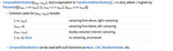
CensoredDistribution[{x_min,x_max},dist]はTransformedDistribution[f,xdist]に等しい．ただし，f はPiecewise[{{x_min,x<=x_min},{x,x_min<x<x_max},{x_max,x>=x_max}}]で与えられる．
{x_min,x_max}によく使われるケース

	{-∞,x_max}	上から打切り，右打切り
	{x_min,∞}	下から打切り，左打切り
	{x_min,x_max}	両側打切り，区間打切り
	{-∞,∞},None	打切りなし

CensoredDistributionは，Mean，CDF，RandomVariate等の関数とともに使うことができる．

予備知識

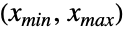
CensoredDistribution[{x_min,x_max},dist]は，区間におけるすべてのについての一様分布 dist から取られたことが分かっており，について（については）と常に等しいと仮定されるデータをモデル化する統計分布を表す．打切りなし，左打切り，右打切り，両側打切りという用語は，{x_min,x_max}がそれぞれ {-∞,∞}，{x_min,∞}，{-∞,x_max}，{x_min,x_max}の形である一変量の打切り分布を説明するために使われるのに対し，一変量分布 dist は，TransformedDistribution，CensoredDistribution，TruncatedDistributionを使った既知の分布の変換，打切りあるいは切断によって定義できる連続分布（例：NormalDistribution，GammaDistribution，BetaDistribution）あるいは離散分布（例：PoissonDistribution，BinomialDistribution，BernoulliDistribution）を示す．
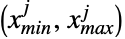
多変量打切り分布CensoredDistribution[{{,},{,},… ,{,}},dist]は一変量分布と同じように定義された，多変量分布 dist から取られ，区間内に収まるように第成分が打ち切られたベクトルの分布を表す．一変量の場合と同じように，多変量分布 dist にも連続分布（例：MultinormalDistribution）と離散分布（例：MultivariateHypergeometricDistribution）があり，（それぞれCopulaDistributionおよびProductDistributionを使って）既知の分布のコピュラ分布あるいは積分布として定義できることがある．
打切り分布は，値が部分的にしか分からないデータ（つまり，部分的に観測されたデータあるい確度に制約条件が課されているデータ）のモデル化で使われる．打切り値を含むデータ集合の分析は18世紀におけるDaniel Bernoulliの天然痘の研究まで遡ることができる．このようなデータは，医学，生理学等や，失敗予測が実際の失敗を観測することなしに行われる信頼性や製造業の分野で比較的よく見られる．打切り分布は生存分析でもよく使われるツールで，そのようなデータ集合の分析用に特化された統計ツール（例：打切り回帰）が存在する．
定義により，CensoredDistribution[{x_min,x_max},dist]はTransformedDistribution[f,xdist]に等しい．ただし，f はPiecewise[{{x_min,x<=x_min},{x,x_min<x<x_max},{x_max,x>=x_max}}]によって与えられる．CensoredDistributionはしばしばTruncatedDistributionと混同されることがあるが，打切り分布が打切り区間の終りに確率を置くのに対し切断分布はその区間全体に確率を分布させる点で，両者は根本的に異なる．

例題

すべて開くすべて閉じる

例 (2)

左側打切り離散分布を定義する：

Wolfram Language code: 𝒟 = CensoredDistribution[{5, ∞}, 𝒹 = BinomialDistribution[10, .6]];

累積分布関数：

Wolfram Language code: DiscretePlot[{PDF[𝒹, x], PDF[𝒟, x]}//Evaluate, {x, 0, 12}, ExtentSize -> 1 / 2, PlotLegends -> {"𝒹", "𝒟"}]

右側打切り連続分布を定義する：

Wolfram Language code: 𝒟 = CensoredDistribution[{-∞, 2}, 𝒩 = NormalDistribution[1, 2]];

累積分布関数：

Wolfram Language code:

Plot[CDF[First[#], x]//Evaluate, {x, -4, 7}, Exclusions -> None, Filling -> Axis, PlotLabel -> Last[#]]& /@ {{𝒟, "𝒟"}, {𝒩, "𝒩"}}

スコープ (26)

基本的な用法 (9)

一変量離散分布のさまざまな打切りタイプを定義する：

Wolfram Language code:

LeftCensored𝒟 = CensoredDistribution[{5, ∞}, PoissonDistribution[7]];
RightCensored𝒟 = CensoredDistribution[{-∞, 9}, PoissonDistribution[7]];
DoubleCensored𝒟 = CensoredDistribution[{5, 9}, PoissonDistribution[7]];

Wolfram Language code:

Table[DiscretePlot[{PDF[m, x], PDF[PoissonDistribution[7], x]}//Evaluate, {x, 0, 13}, ExtentSize -> 0.5], {m, {LeftCensored𝒟, RightCensored𝒟, DoubleCensored𝒟}}]

一変量連続分布のさまざまな打切りタイプを定義する：

Wolfram Language code:

LeftCensored𝒟 = CensoredDistribution[{-1, ∞}, NormalDistribution[]];
RightCensored𝒟 = CensoredDistribution[{-∞, 1}, NormalDistribution[]];
DoubleCensored𝒟 = CensoredDistribution[{-1, 1}, NormalDistribution[]];

Wolfram Language code:

Table[Plot[{CDF[m, x], CDF[NormalDistribution[], x]}, {x, -3, 3}, Filling -> Axis, Exclusions -> None], {m, {LeftCensored𝒟, RightCensored𝒟, DoubleCensored𝒟}}]

右側打切り離散分布を定義する：

Wolfram Language code: 𝒟 = CensoredDistribution[{0, 9}, 𝒹 = BinomialDistribution[12, .7]];

確率密度関数を比較する：

Wolfram Language code: DiscretePlot[{PDF[𝒹, x], PDF[𝒟, x]}, {x, 3, 13}, ExtentSize -> 1 / 2, PlotLegends -> {"𝒹", "𝒟"}]

打切り分布の9における確率を求める：

Wolfram Language code: PDF[𝒟, 9]

もとの分布で値が少なくとも9になる確率を比較する：

Wolfram Language code: Probability[x ≥ 9, x𝒹]

連続分布を打ち切る：

Wolfram Language code: 𝒟 = CensoredDistribution[{-1, ∞}, NormalDistribution[]];

Wolfram Language code: CDF[𝒟, x]

ヒストグラムを使ってもとの密度関数をプロットし，点確率を可視化する：

Wolfram Language code:

Show[Histogram[RandomVariate[𝒟, 10 ^ 3], {-3, 3, .2}, "PDF"], Plot[PDF[NormalDistribution[], x], {x, -3, 3}, PlotStyle -> Thick]]

1点で打ち切られた分布：

Wolfram Language code: 𝒟1 = CensoredDistribution[{2, 2}, BinomialDistribution[3, .4]];

Wolfram Language code: PDF[𝒟1, x]

Wolfram Language code: 𝒟2 = CensoredDistribution[{2, 2}, ParetoDistribution[1, 1 / 3]];

Wolfram Language code: CDF[𝒟2, x]

多変量連続分布の打切り：

Wolfram Language code: 𝒟 = CensoredDistribution[{{1 / 3, 1 / 2}, {2 / 5, 4 / 5}}, DirichletDistribution[{1, 3, 2}]];

この分布の式の期待値を計算する：

Wolfram Language code: NExpectation[x ^ 2 + y, {x, y}𝒟]

多変量離散分布の打切り：

Wolfram Language code: 𝒟 = CensoredDistribution[{{2, 10}, {4, 12}, {3, 19}}, MultinomialDistribution[20, {1 / 3, 1 / 2, 1 / 6}]];

分布の平均を計算する：

Wolfram Language code: Mean[𝒟]//N

分布から無作為にサンプルを抽出することで得た結果と比較する：

Wolfram Language code: data = RandomVariate[𝒟, 10 ^ 4];

Wolfram Language code: Mean[data]//N

両側打切り分布を定義する：

Wolfram Language code: 𝒟 = CensoredDistribution[{1.2, 2}, 𝒹 = TriangularDistribution[{0, 4}]];

累積分布関数：

Wolfram Language code:

Plot[{CDF[𝒹, x], CDF[𝒟, x]}//Evaluate, {x, 0, 5 / 2}, PlotStyle -> {Automatic, Thick}, Filling -> {2 -> Axis}, Exclusions -> None, PlotLegends -> {"𝒹", "𝒟"}]

打切り分布の平均と分散：

Wolfram Language code: {Mean[𝒟], Variance[𝒟]}

Momentは記号次数で閉形式を持つ：

Wolfram Language code: Moment[𝒟, r]

打切り区間を推定する：

Wolfram Language code: data = RandomVariate[CensoredDistribution[{2, 7}, PoissonDistribution[5]], 10 ^ 2];

Wolfram Language code: edist = EstimatedDistribution[data, CensoredDistribution[{a, b}, PoissonDistribution[5]]]

パラメトリック分布 (5)

右打切り連続分布を定義する：

Wolfram Language code: 𝒟 = CensoredDistribution[{0, 1 / 2}, BetaDistribution[2, 3]];

累積分布関数：

Wolfram Language code: CDF[𝒟, x]

ランダムなサンプルのヒストグラムをプロットする．峰はPDFのDiracDelta部分に対応する：

Wolfram Language code:

Show[Histogram[RandomVariate[𝒟, 10 ^ 3], Automatic, "PDF"], Plot[PDF[𝒟, x]//Evaluate, {x, 0, 1}, PlotStyle -> Thick, Exclusions -> None]]

打切りGeometricDistributionを定義する：

Wolfram Language code: 𝒟 = CensoredDistribution[{2, 5}, 𝒹 = GeometricDistribution[.2]];

確率密度関数を比較する：

Wolfram Language code: DiscretePlot[{PDF[𝒹, x], PDF[𝒟, x]}//Evaluate, {x, 0, 10}, ExtentSize -> 1 / 2, PlotLegends -> {"𝒹", "𝒟"}]

Wolfram Language code: PDF[𝒟, x]

打切り点における確率密度関数の値は次の確率に等しい：

Wolfram Language code: {Probability[x ≤ 2, x𝒹], PDF[𝒟, 2]}

Wolfram Language code: {Probability[x ≥ 5, x𝒹], PDF[𝒟, 5]}

両側打切りGammaDistributionを定義する：

Wolfram Language code: 𝒟 = CensoredDistribution[{2, 4}, GammaDistribution[2, 1]];

母関数を求める：

Wolfram Language code: CharacteristicFunction[𝒟, t]//FullSimplify

Wolfram Language code: MomentGeneratingFunction[𝒟, t]//FullSimplify

Wolfram Language code: CumulantGeneratingFunction[𝒟, t]//FullSimplify

Wolfram Language code: FactorialMomentGeneratingFunction[𝒟, t]//FullSimplify

右側打切りPoissonDistributionを定義する：

Wolfram Language code: 𝒟 = CensoredDistribution[{-∞, 7}, 𝒫 = PoissonDistribution[5]];

HazardFunctionを比較する：

Wolfram Language code: DiscretePlot[{HazardFunction[𝒫, x], HazardFunction[𝒟, x]}, {x, 0, 9}, PlotRange -> All, ExtentSize -> 1 / 2]

二次元打切りDirichletDistributionを定義する：

Wolfram Language code: 𝒟 = CensoredDistribution[{{1 / 3, 1 / 2}, {1 / 3, 3 / 5}}, 𝒹 = DirichletDistribution[{3, 2, 4}]];

累積分布関数を比較する：

Wolfram Language code:

Plot3D[CDF[#, {x, y}]//Evaluate, {x, -1 / 10, 3 / 4}, {y, -1 / 10, 4 / 5}, PlotRange -> All, AxesLabel -> Automatic, Exclusions -> None]&  /@ {𝒹, 𝒟}

打切り分布の平均と分散：

Wolfram Language code: Mean[𝒟]

Wolfram Language code: Variance[𝒟]

確率と期待値を計算する：

Wolfram Language code: NProbability[2 / 5 < x < 23 / 50 && y > 2 / 5, {x, y}𝒟]

Wolfram Language code: NExpectation[x ^ 3 + y ^ 3, {x, y}𝒟]

ノンパラメトリック分布 (3)

打切りEmpiricalDistributionを定義する：

Wolfram Language code:

ed = EmpiricalDistribution[RandomVariate[WeibullDistribution[2, 3], 15]];
𝒟 = CensoredDistribution[{0, 2}, ed];

累積分布関数を比較する：

Wolfram Language code:

Plot[{CDF[ed, x], CDF[𝒟, x]}, {x, 0, 6}, Filling -> Axis, PlotStyle -> {Automatic, Thick}, Exclusions -> None, PlotLegends -> {"ed", "𝒟"}]

打切りHistogramDistributionを定義する：

Wolfram Language code:

hd = HistogramDistribution[RandomVariate[PoissonDistribution[6], 10 ^ 3]];
𝒟 = CensoredDistribution[{0, 6}, hd];

累積分布関数を比較する：

Wolfram Language code:

Plot[{CDF[hd, x], CDF[𝒟, x]}, {x, 0, 12}, Filling -> Axis, Exclusions -> None, PlotStyle -> {Automatic, Thick}, PlotLegends -> {"hd", "𝒟"}]

打切りSmoothKernelDistributionを定義する：

Wolfram Language code:

skd = SmoothKernelDistribution[RandomVariate[LaplaceDistribution[0, 2], 10 ^ 3]];
𝒟 = CensoredDistribution[{-1, 1}, skd];

累積分布関数を比較する：

Wolfram Language code:

Plot[{CDF[skd, x], CDF[𝒟, x]}, {x, -3, 3}, Filling -> Axis, PlotStyle -> {Automatic, Thick}, Exclusions -> None, PlotLegends -> {"skd", "𝒟"}]

派生分布 (9)

打切りParameterMixtureDistributionを定義する：

Wolfram Language code:

ℳ = ParameterMixtureDistribution[GammaDistribution[1 / 2, β], βUniformDistribution[{1, 2}]];
𝒟 = CensoredDistribution[{0, 1}, ℳ];

累積分布関数：

Wolfram Language code: CDF[𝒟, x]

Wolfram Language code:

Plot[CDF[First[#], x]//Evaluate, {x, 0, 2}, Filling -> Axis, Exclusions -> None, PlotLabel -> Last[#]]& /@ {{ℳ, "ℳ"}, {𝒟, "𝒟"}}

打切りMixtureDistributionを定義する：

Wolfram Language code:

ℳ = MixtureDistribution[{1, 2}, {NormalDistribution[-1, 3], NormalDistribution[1, 2]}];
𝒟 = CensoredDistribution[{-2, 2}, ℳ];

累積分布関数：

Wolfram Language code: CDF[𝒟, x]

Wolfram Language code:

Plot[Evaluate[CDF[First[#], x]], {x, -3, 3}, Filling -> Axis, Exclusions -> None, PlotLabel -> Last[#]]& /@ {{ℳ, "ℳ"}, {𝒟, "𝒟"}}

打切りOrderDistributionを定義する：

Wolfram Language code:

𝒫 = OrderDistribution[{BinomialDistribution[10, 0.6], 4}, 1];
𝒟 = CensoredDistribution[{4, ∞}, 𝒫];

確率密度関数：

Wolfram Language code: DiscretePlot[{PDF[𝒫, x], PDF[𝒟, x]}, {x, 0, 10}, ExtentSize -> 1 / 2, PlotLegends -> {"𝒫", "𝒟"}]

平均を比較する：

Wolfram Language code: {Mean[𝒟], Mean[𝒫]}

打切りCensoredDistributionを定義する：

Wolfram Language code:

𝒞 = CensoredDistribution[{-∞, 9}, 𝒫 = PoissonDistribution[7]];
𝒟 = CensoredDistribution[{6, ∞}, 𝒞];

確率密度関数：

Wolfram Language code:

DiscretePlot[Evaluate[PDF[First[#], x]], {x, 0, 15}, ExtentSize -> 1 / 2, PlotLabel -> Last[#]]& /@ {{𝒫, "𝒫"}, {𝒞, "𝒞"}, {𝒟, "𝒟"}}

Wolfram Language code: PDF[𝒟, x]

両側打切りポアソン分布と比較する：

Wolfram Language code: PDF[CensoredDistribution[{6, 9}, PoissonDistribution[7]], x]

Wolfram Language code: % - %%

打切りTruncatedDistributionを定義する：

Wolfram Language code:

𝒯 = TruncatedDistribution[{-∞, 1}, 𝒩 = NormalDistribution[0, 2]];
𝒟 = CensoredDistribution[{-1, ∞}, 𝒯];

累積分布関数を比較する：

Wolfram Language code:

Plot[Evaluate[CDF[First[#], x]], {x, -3, 3}, Filling -> Axis, Exclusions -> None, PlotLabel -> Last[#]]& /@ {{𝒩, "𝒩"}, {𝒯, "𝒯"}, {𝒟, "𝒟"}}

打切りTransformedDistributionを定義する：

Wolfram Language code:

𝒯 = TransformedDistribution[u + 1, uBenfordDistribution[10]];
𝒟 = CensoredDistribution[{3, 6}, 𝒯];

累積分布関数：

Wolfram Language code: CDF[𝒟, x]

打切りMarginalDistributionを定義する：

Wolfram Language code:

ℳ = MarginalDistribution[NegativeMultinomialDistribution[3, {1 / 3, 1 / 3, 1 / 6}], 1];
𝒟 = CensoredDistribution[{3, 10}, ℳ];

確率密度関数：

Wolfram Language code: pdf = PDF[𝒟, x]

周辺分布の確率密度関数と比較する：

Wolfram Language code: DiscretePlot[{PDF[ℳ, x], pdf}, {x, 0, 15}, ExtentSize -> 1 / 2, PlotLegends -> {"ℳ", "𝒟"}]

打切りProductDistributionを定義する：

Wolfram Language code:

𝒫 = ProductDistribution[PoissonDistribution[8], PoissonDistribution[9]];
𝒟 = CensoredDistribution[{{-∞, 12}, {5, ∞}}, 𝒫];

ランダムなサンプルを使って密度関数を可視化する：

Wolfram Language code: Histogram3D[RandomVariate[𝒟, 10 ^ 4], 20, "PDF"]

QuantityDistributionの打切り分布を評価するとQuantityDistributionになる：

Wolfram Language code:

𝒟 = CensoredDistribution[{-∞, Quantity[75, "Miles"/"Hours"]}, QuantityDistribution[NormalDistribution[70, 8], "mph"]]

平均速度を計算する：

Wolfram Language code: Mean[𝒟]//N

アプリケーション (4)

保険会社が保有レベルで再保険を買う．保険金請求が対数正規分布に従うと仮定して，保険会社の支払い確率変量を求める：

Wolfram Language code: Refine[Moment[CensoredDistribution[{0, M}, LogNormalDistribution[μ, σ]], n], M > 0 && σ > 0]

再保険をかけた会社の支払い確率変量のモーメントを求める：

Wolfram Language code: Refine[Moment[CensoredDistribution[{M, Infinity}, LogNormalDistribution[μ, σ]], n], M > 0 && σ > 0]

ある部品の寿命がRayleighDistributionに従う．この部品は故障するかどうかを見るために時間テストされる．テスト後でも故障していなければ，この部品の寿命は厳密に時間であると想定される．テストされた部品の寿命がより長くなる確率が最高で5%になるようなテスト時間を求める：

Wolfram Language code: component𝒟 = RayleighDistribution[Quantity[3, "Hours"]]

Wolfram Language code: Solve[CDF[component𝒟, n] == 95 / 100, n]

Wolfram Language code: N[%]

について検証寿命の分布を求める：

Wolfram Language code: test𝒟 = CensoredDistribution[{Quantity[0, "Hours"], Quantity[7.35, "Hours"]}, component𝒟];

実際の寿命分布と打ち切られた寿命分布を比較する：

Wolfram Language code:

Plot[{CDF[component𝒟, Quantity[x, "Hours"]], CDF[test𝒟, Quantity[x, "Hours"]]}, {x, 0, 10}, Filling -> 1 -> {2}, Epilog -> {Dashed, Line[{{7.35, 0}, {7.35, 1}}]}, PlotLegends -> {"component𝒟", "test𝒟"}, AxesLabel -> {"h"}]

平均寿命を比べる：

Wolfram Language code: Mean /@ {component𝒟, test𝒟}//N

パー4のホールでのゴルフ初心者の打数は平均9打でPoissonDistributionに従う．あるゴルフコースでこのゴルファーが10打でホールアウトしたとしてパー4のホールの打数の平均を求める：

Wolfram Language code: 𝒟 = TransformedDistribution[u + 1, uCensoredDistribution[{0, 9}, PoissonDistribution[8]]];

確率密度関数：

Wolfram Language code: DiscretePlot[Evaluate[PDF[𝒟, x]], {x, 0, 11}, ExtentSize -> 1 / 2]

Wolfram Language code: PDF[𝒟, x]

ゴルフコースのパー4のホールでの平均打数：

Wolfram Language code: Mean[𝒟]//N

この人がボールを沈めるまでに4打以上必要な確率を求める：

Wolfram Language code: NProbability[x > 4, x𝒟]

アメリカ合衆国の成人男性の体重は平均191ポンド，標準偏差70ポンドで正規分布に従う．体重計の上限が300ポンドだと仮定して，一般的な体重計で計った場合の体重分布を求める：

Wolfram Language code:

𝒟 = CensoredDistribution[{Quantity[0, "Pounds"], Quantity[300, "Pounds"]}, 𝒹 = NormalDistribution[Quantity[191, "Pounds"], Quantity[70, "Pounds"]]];

累積分布関数：

Wolfram Language code: Plot[Evaluate[CDF[𝒟, Quantity[x, "Pounds"]]], {x, 0, 350}, Filling -> Axis, Exclusions -> None, AxesLabel -> {"lbs"}]

ランダムなサンプルを使って密度関数を可視化する：

Wolfram Language code: Histogram[RandomVariate[𝒟, 10 ^ 5], Automatic, "PDF", AxesLabel -> Automatic]

平均体重を求める：

Wolfram Language code: Mean[𝒟]//N

体重が少なくとも200ポンドある確率を求める：

Wolfram Language code: NProbability[x ≥ Quantity[200, "Pounds"], x𝒟]

体重が体重計の上限以上である確率を求める：

Wolfram Language code: Probability[x ≥ Quantity[300, "Pounds"], x𝒟]//N

打切りのない分布と比較する：

Wolfram Language code: Probability[x ≥ Quantity[300, "Pounds"], x𝒹]//N

特性と関係 (4)

CensoredDistributionはTransformedDistributionの特殊ケースである：

Wolfram Language code:

𝒟1 = CensoredDistribution[{2, 3}, NormalDistribution[]];
𝒟2 = TransformedDistribution[Piecewise[{{2, u ≤ 2}, {u, 2 ≤ u ≤ 3}, {3, u > 3}}], uNormalDistribution[]];

Wolfram Language code: CDF[𝒟1, x]

Wolfram Language code: CDF[𝒟2, x]

Wolfram Language code: % - %%//FullSimplify

離散分布で打切りと切断を比較する：

Wolfram Language code:

𝒞 = CensoredDistribution[{4, 9}, 𝒫 = PoissonDistribution[7]];
𝒯 = TruncatedDistribution[{4, 9}, 𝒫];

打切りでは外部からの重みが打切り区間の末尾に置かれる：

Wolfram Language code: DiscretePlot[{PDF[𝒫, x], PDF[𝒞, x]}, {x, 0, 12}, ExtentSize -> 1 / 2, PlotLegends -> {"𝒫", "𝒞"}]

切断では，外部からの重みが切断区間に等しく分布される：

Wolfram Language code: DiscretePlot[{PDF[𝒫, x], PDF[𝒯, x]}, {x, 0, 12}, ExtentSize -> 1 / 2, PlotLegends -> {"𝒫", "𝒯"}]

連続分布の打切りと切断を比較する：

Wolfram Language code:

𝒞 = CensoredDistribution[{1 / 2, ∞}, 𝒩 = NormalDistribution[0, 1 / 2]];
𝒯 = TruncatedDistribution[{1 / 2, ∞}, 𝒩];

打切りでは，確率が打切り区間の末尾に置かれる：

Wolfram Language code: Plot[{CDF[𝒩, x], CDF[𝒞, x]}, {x, -2, 3}, Filling -> Axis, PlotLegends -> {"𝒩", "𝒞"}]

切断では，確率が切断区間全体に分布される：

Wolfram Language code: Plot[{CDF[𝒩, x], CDF[𝒯, x]}, {x, -2, 3}, Filling -> Axis, PlotLegends -> {"𝒩", "𝒯"}]

連続分布を打ち切ると，連続的でも離散的でもない混合分布になることがある：

Wolfram Language code:

cont𝒟 = LogisticDistribution[];
cens𝒟 = CensoredDistribution[{-1, 1}, cont𝒟]

混合タイプの打切り分布のCDFは打切り点で不連続である：

Wolfram Language code: cdf = CDF[cens𝒟, x]

累積分布関数を可視化する：

Wolfram Language code:

ticks = {{-1, -0.5, 0, 0.5, 1}, {0, {CDF[cont𝒟, -1], HoldForm[F[-1 + ϵ]]}, 0.5, {CDF[cont𝒟, 1], HoldForm[F[1 - ϵ]]}, 1}};
Plot[{cdf, Style[CDF[cont𝒟, x], DotDashed]}, {x, -1.75, 1.75}, Ticks -> ticks, ExclusionsStyle -> {Directive[Dotted, Red], PointSize[Medium]}, PlotLegends -> {"censored 𝒟", "underlying continuous 𝒟"}]

打切り分布の確率密度関数は定義されず，PDFは未評価で返される：

Wolfram Language code: PDF[cens𝒟, x]

累積分布関数を微分すると結果として積分しても1にならない関数になる：

Wolfram Language code: D[cdf, x]

Wolfram Language code: NIntegrate[D[cdf, x], {x, -∞, ∞}]

確率密度推定器のサンプルは，サンプルサイズが大きくなるにつれて収束しなくなる：

Wolfram Language code:

Table[Labeled[Histogram[RandomVariate[cens𝒟, 10 ^ k], "Scott", "PDF", ImageSize -> Small], Row[{Text@"Sample size", ":", HoldForm[10] ^ k//TraditionalForm}]], {k, {3, 6}}]

これを，推定器が収束するもとになっている連続分布のヒストグラムと比較する：

Wolfram Language code:

Table[Labeled[Histogram[RandomVariate[cont𝒟, 10 ^ k], "Scott", "PDF", ImageSize -> Small], Row[{Text@"Sample size", ":", HoldForm[10] ^ k//TraditionalForm}]], {k, {3, 6}}]

考えられる問題 (1)

連続分布を打ち切ると連続的でも離散的でもない混合分布になる可能性がある：

Wolfram Language code:

cont𝒟 = NormalDistribution[];
cens𝒟 = CensoredDistribution[{-1, 1}, cont𝒟]

混合型の打切り分布のCDFは定義されない： »

Wolfram Language code: PDF[cens𝒟, x]

混合型分布の計算は完全にサポートされている．特殊なモーメントを計算する：

Wolfram Language code: {Mean[cens𝒟], Variance[cens𝒟], Skewness[cens𝒟], Kurtosis[cens𝒟]}

打切り分布を推定する：

Wolfram Language code: sample = RandomVariate[cens𝒟, 10 ^ 4];

Wolfram Language code: EstimatedDistribution[sample, CensoredDistribution[{min, max}, NormalDistribution[μ, σ]]]

混合型分布は連続分布と離散分布の混合と解釈することができる：

Wolfram Language code: ProbabilityDistribution[{CDF, CDF[cens𝒟, x]}, {x, -Infinity, Infinity}]//FullSimplify

Top

その他のラーニングリソース

テクニカルサポート

Wolframソリューション

教育のためのWolframソリューション

使い始める

Grow Your Skills

Wolframと繋がる

大人用の教育プログラム

若者のための教育プログラム

読む

CensoredDistribution

詳細

予備知識

例題

例 (2)

スコープ (26)

基本的な用法 (9)

パラメトリック分布 (5)

ノンパラメトリック分布 (3)

派生分布 (9)

アプリケーション (4)

特性と関係 (4)

考えられる問題 (1)

テキスト

CMS

APA

BibTeX

BibLaTeX

CensoredDistribution

詳細

予備知識

例題

例 (2)

スコープ (26)

基本的な用法 (9)

パラメトリック分布 (5)

ノンパラメトリック分布 (3)

派生分布 (9)

アプリケーション (4)

特性と関係 (4)

考えられる問題 (1)

関連項目

関連するガイド

履歴

テキスト

CMS

APA

BibTeX

BibLaTeX