

GeometricDistribution
represents a geometric distribution with probability parameter p.
Details
- The probability for value
 in a geometric distribution is
  for non-negative integers, and is zero otherwise. »
 - GeometricDistribution[p] is the distribution of the number of failures in a sequence of trials with success probability p before a success occurs.
- GeometricDistribution allows p to be a dimensionless quantity. »
- GeometricDistribution can be used with such functions as Mean, CDF, and RandomVariate. »
Background & Context
- GeometricDistribution[p] represents a discrete statistical distribution defined at integer values
 and parametrized by a non-negative real number
  . The geometric distribution has a discrete probability density function (PDF) that is monotonically decreasing, with the parameter p determining the height and steepness of the PDF. The geometric distribution is sometimes referred to as the Furry distribution.
 - The geometric distribution is sometimes said to be the discrete analog of the exponential distribution (ExponentialDistribution). It can be defined as the distribution that models the number of Bernoulli trials (i.e. number of trials of a variate having a BernoulliDistribution) needed to obtain a single success. The geometric distribution has been used to model a number of different phenomena across many fields, including the behavior of competing plant populations, dynamics of ticket control, particulars of congenital malformations, and estimation of animal abundance. Moreover, the geometric distribution has been used widely in reliability theory and is a staple in Markov chain models for meteorology, queueing theory, and applied stochastics.
- RandomVariate can be used to give one or more machine- or arbitrary-precision (the latter via the WorkingPrecision option) pseudorandom variates from a geometric distribution. Distributed[x,GeometricDistribution[p]], written more concisely as xGeometricDistribution[p], can be used to assert that a random variable x is distributed according to a geometric distribution. Such an assertion can then be used in functions such as Probability, NProbability, Expectation, and NExpectation.
- The probability density and cumulative distribution functions may be given using PDF[GeometricDistribution[p],x] and CDF[GeometricDistribution[p],x]. The mean, median, variance, raw moments, and central moments may be computed using Mean, Median, Variance, Moment, and CentralMoment, respectively. These quantities can be visualized using DiscretePlot.
- DistributionFitTest can be used to test if a given dataset is consistent with a geometric distribution, EstimatedDistribution to estimate a geometric parametric distribution from given data, and FindDistributionParameters to fit data to a geometric distribution. ProbabilityPlot can be used to generate a plot of the CDF of given data against the CDF of a symbolic geometric distribution and QuantilePlot to generate a plot of the quantiles of given data against the quantiles of a symbolic geometric distribution.
- TransformedDistribution can be used to represent a transformed geometric distribution, CensoredDistribution to represent the distribution of values censored between upper and lower values, and TruncatedDistribution to represent the distribution of values truncated between upper and lower values. CopulaDistribution can be used to build higher-dimensional distributions that contain a geometric distribution, and ProductDistribution can be used to compute a joint distribution with independent component distributions involving geometric distributions.
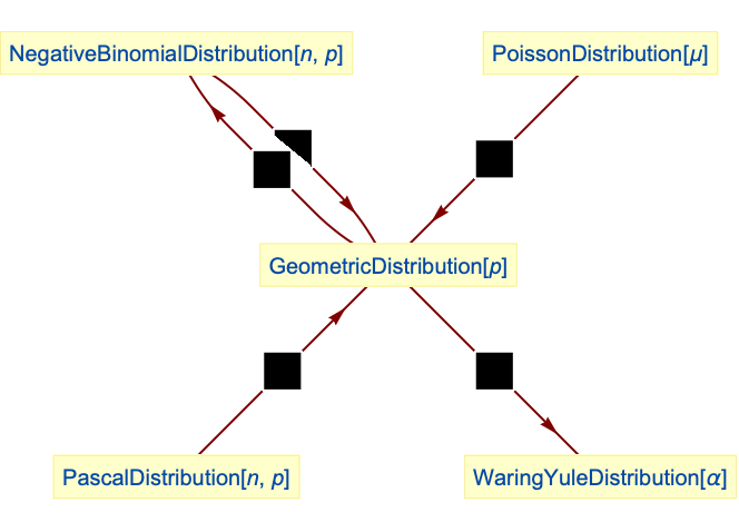
- GeometricDistribution is related to a number of other statistical distributions. For example, GeometricDistribution is a special case of the more general NegativeBinomialDistribution, in the sense that NegativeBinomialDistribution[1,p] has precisely the same PDF as GeometricDistribution[p] and that the sum of
 is distributed according to NegativeBinomialDistribution[n,p], provided that XiGeometricDistribution[p] for all
  . GeometricDistribution is also a transformation of PascalDistribution and can be viewed as a parameter mixture of PoissonDistribution with either GammaDistribution or ExponentialDistribution, in the sense that both ParameterMixtureDistribution[PoissonDistribution[μ],μGammaDistribution[1,(1-p)/p]] and ParameterMixtureDistribution[PoissonDistribution[μ],μ ExponentialDistribution[p/(1-p)]] are the same as GeometricDistribution[p]. GeometricDistribution is also related to WaringYuleDistribution, BinomialDistribution, PascalDistribution, and HypergeometricDistribution.
Examples
open all close allBasic Examples (3)
DiscretePlot[Table[PDF[GeometricDistribution[p], k], {p, {0.1, 0.2, 0.4}}]//Evaluate, {k, 15}, PlotMarkers -> Automatic, PlotRange -> All]PDF[GeometricDistribution[p], k]Cumulative distribution function:
DiscretePlot[Table[CDF[GeometricDistribution[p], k], {p, {0.1, 0.2, 0.5}}]//Evaluate, {k, 0, 14}, ExtentSize -> Right]CDF[GeometricDistribution[p], k]Mean and variance of a geometric distribution:
Mean[GeometricDistribution[p]]Variance[GeometricDistribution[p]]Scope (8)
Generate a sample of pseudorandom numbers from a geometric distribution:
data = RandomVariate[𝒹 = GeometricDistribution[.1], 10 ^ 4];Compare its histogram to the PDF:
Show[
	Histogram[data, {2}, "PDF"],
	DiscretePlot[PDF[𝒹, x], {x, 0, 40}, PlotStyle -> PointSize[Medium]]]
Distribution parameters estimation:
sample = RandomVariate[GeometricDistribution[.3], 10 ^ 3];Estimate the distribution parameters from sample data:
edist = EstimatedDistribution[sample, GeometricDistribution[p]]Compare the density histogram of the sample with the PDF of the estimated distribution:
Show[Histogram[sample, {1}, "PDF"], DiscretePlot[PDF[edist, x], {x, 0, 15}, PlotStyle -> PointSize[Medium]]]Plot[Skewness[GeometricDistribution[p]], {p, 0, 1}, Filling -> Axis]Skewness[GeometricDistribution[p]]Limit[Skewness[GeometricDistribution[p]], p -> 0]Limit[Skewness[GeometricDistribution[p]], p -> 1, Direction -> 1]Plot[Kurtosis[GeometricDistribution[p]], {p, 0, 1}, Filling -> Axis]Kurtosis[GeometricDistribution[p]]Limit[Kurtosis[GeometricDistribution[p]], p -> 0]Limit[Kurtosis[GeometricDistribution[p]], p -> 1, Direction -> 1]Different moments with closed forms as functions of parameters:
FormulaGrid[list_, type_] := Grid[...]FormulaGrid[Table[Moment[GeometricDistribution[p], k]//Together, {k, 3}], M]Closed form for symbolic order:
Moment[GeometricDistribution[p], r]FormulaGrid[Table[CentralMoment[GeometricDistribution[p], k]//Together, {k, 3}], CM]Closed form for symbolic order:
CentralMoment[GeometricDistribution[p], r]FormulaGrid[Table[FactorialMoment[GeometricDistribution[p], k], {k, 3}], FM]Closed form for symbolic order:
FactorialMoment[GeometricDistribution[p], r]FormulaGrid[Table[Cumulant[GeometricDistribution[p], k]//Together, {k, 3}], C]HazardFunction[GeometricDistribution[p], x]𝒟 = GeometricDistribution[.3];
points = N[Table[CDF[𝒟, x], {x, 0, 6}]];DiscretePlot[Quantile[𝒟, p], {p, points}, ExtentSize -> Right, ExtentMarkers -> {"Empty", "Filled"}]Use dimensionless Quantity to define GeometricDistribution:
𝒟 = GeometricDistribution[Quantity[25, "Percent"]]Applications (11)
CDF of GeometricDistribution is an example of a right-continuous function:
DiscretePlot[CDF[GeometricDistribution[.7], x], {x, 0, 4}, ExtentSize -> Right, ExtentMarkers -> {"Filled", "Empty"}]A coin-tossing experiment consists of tossing a fair coin repeatedly until a tail results. Simulate the process:
RandomVariate[GeometricDistribution[1 / 2], 10]ListPlot[RandomVariate[GeometricDistribution[1 / 2], 100], Filling -> Axis]Compute the probability that at least 4 coin tosses will be necessary:
Probability[x ≥ 4, xGeometricDistribution[1 / 2]]Compute the expected number of coin tosses:
Mean[GeometricDistribution[1 / 2]]A person is standing by a road counting cars until he sees a red one, at which point he restarts the count. Simulate the counting process, assuming that 20% of the cars are red:
RandomVariate[GeometricDistribution[0.2], 20]ListPlot[%, Filling -> Axis]Find the expected number of cars to come by before the count starts over:
Mean[GeometricDistribution[0.2]]Find the probability of counting 10 or more cars before a red one:
NProbability[x ≥ 10, xGeometricDistribution[0.2]]A student will take a test repeatedly until he or she passes it, each time succeeding with probability p. Find the probability that the student succeeds in ![]() attempts or less:
attempts or less:
prob1 = Probability[x ≤ k, xGeometricDistribution[p], Assumptions -> k∈Integers && k ≥ 0]Block[{p = 1 / 3}, DiscretePlot[prob1, {k, 10}]]Given that the student passes the test in ![]() attempts or less, find the PDF:
attempts or less, find the PDF:
prob2 = Probability[x == kx ≤ n, xGeometricDistribution[p], Assumptions -> {k, n}∈Integers && n > 0]//FullSimplifyBlock[{p = 1 / 3, n = 3}, DiscretePlot[prob2, {k, 10}]]A budget-priced lighter has 90% probability of lighting on any given attempt. Simulate the lighting process; the result indicates the number of failures before successful lighting:
BarChart[RandomVariate[GeometricDistribution[Quantity[90, "Percent"]], 100]]Find the probability that the lighter lights in 3 trials or less:
NProbability[x ≤ 3, xGeometricDistribution[Quantity[90, "Percent"]]]A cereal box contains one out of a set of ![]() different plastic animals. The animals are equally likely to occur, independently of what animals are in other boxes. Simulate the animal collection process, assuming there are 10 animals for 25 boxes:
different plastic animals. The animals are equally likely to occur, independently of what animals are in other boxes. Simulate the animal collection process, assuming there are 10 animals for 25 boxes:
RandomVariate[DiscreteUniformDistribution[{1, 10}], 25]After ![]() unique animals have been collected, the number of boxes needed to find a new unique animal among the remaining
unique animals have been collected, the number of boxes needed to find a new unique animal among the remaining ![]() follows a geometric distribution with parameter
follows a geometric distribution with parameter ![]() . Find the expected number of boxes needed to get a new unique animal:
. Find the expected number of boxes needed to get a new unique animal:
e = Expectation[x + 1, xGeometricDistribution[1 - k / n]]Number of boxes before next unique animal:
Block[{n = 5}, DiscretePlot[e, {k, 1, n - 1}, ExtentSize -> 1 / 2]]Find the expected number of boxes needed to collect 6 unique animals:
Block[{n = 5}, Sum[e, {k, 0, n - 1}]]N[%]When a computer accesses memory, the desired data is in the cache with probability p. A cache miss occurs if the desired data is not in the cache. Find the probability of a cache miss on the ![]()
![]() memory access:
memory access:
CacheMissDistribution[p_] := TransformedDistribution[a + 1, aGeometricDistribution[1 - p]]Simplify[PDF[CacheMissDistribution[p], k], k∈Integers]Table[PDF[CacheMissDistribution[p], k], {k, 3}]Find the probability that the first cache miss occurs after the 4![]() memory access:
memory access:
Probability[k > 4, kCacheMissDistribution[p]]Find the average number of memory accesses before the first cache miss:
Mean[CacheMissDistribution[p]]Simulate the number of cache hits before a cache miss occurs, assuming 20% of your data is in the cache:
ListPlot[RandomVariate[CacheMissDistribution[0.2], 50], Frame -> True, Filling -> Axis]Assuming that access time is 10 ns for cache and 1000 ns for RAM, find the average access time:
pmiss = PDF[CacheMissDistribution[0.2], 1]Quantity[1000, "ns"] pmiss + Quantity[10, "ns"] (1 - pmiss)A data stream containing ![]() data packets is repeatedly sent without order information. Find the distribution of the number of tries until the data stream arrives with all the packets in the right order for the first time:
data packets is repeatedly sent without order information. Find the distribution of the number of tries until the data stream arrives with all the packets in the right order for the first time:
𝒟 = GeometricDistribution[1 / 4!];PDF[𝒟, x]DiscretePlot[PDF[𝒟, x], {x, 0, 100}]Find the probability that the packets will arrive in the correct order on the 20![]() try or sooner:
try or sooner:
Probability[x ≤ 20, x𝒟]N[%]Simulate the number of tries until the first ordered data stream:
flows = RandomVariate[𝒟, 50]ListPlot[flows, Filling -> Axis]Find the average number of tries until the first ordered data stream:
Mean[𝒟]A player bets amount ![]() in a casino with no betting limit in a game with chance of winning
in a casino with no betting limit in a game with chance of winning ![]() . If he loses he doubles the bet, and if he wins he quits, hence the number of games played follows a geometric distribution, with expected number of games played represented as follows:
. If he loses he doubles the bet, and if he wins he quits, hence the number of games played follows a geometric distribution, with expected number of games played represented as follows:
Expectation[k + 1, kGeometricDistribution[p]]The cash reserve needed to win the ![]()
![]() game:
game:
cashReserve[k_] = Sum[a 2^n - 1, {n, 1, k - 1}]The player always leaves the casino collecting the amount of the initial bet:
a 2^k - 1 - cashReserve[k]//SimplifyThe cash reserve needed to execute the above strategy is finite only for strictly favorable games, where ![]() :
:
Expectation[cashReserve[k + 1], kGeometricDistribution[p], GenerateConditions -> True]In an optical communication system, transmitted light generates current at the receiver. The number of electrons follows the parametric mixture of Poisson distribution and other distributions, depending on the type of light. If the source uses coherent laser light of intensity ![]() , then the electron count distribution is Poisson:
, then the electron count distribution is Poisson:
Bdist = TransformedDistribution[λ x, xBernoulliDistribution[1]];PDF[Bdist, x]//Refine[#, λ > 0]&𝒟1 = ParameterMixtureDistribution[PoissonDistribution[μ], μBdist];PDF[𝒟1, x]Which is PoissonDistribution:
PDF[PoissonDistribution[λ], x]If the source uses thermal illumination, then the Poisson parameter follows ExponentialDistribution with parameter ![]() , and the electron count distribution is:
, and the electron count distribution is:
𝒟2 = ParameterMixtureDistribution[PoissonDistribution[μ], μExponentialDistribution[1 / λ]]These two distributions are distinguishable and allow you to determine the type of source:
Block[{λ = 3}, Histogram[{RandomVariate[𝒟1, 10 ^ 3], RandomVariate[𝒟2, 10 ^ 3]}, {1}, "PDF"]]Find the sampling population expectation of the method of moment estimator for p:
Solve[Mean[GeometricDistribution[p]] == Mean[data], p]{MMEstimator[data_]} = p /. %Find sampling population expectations for a few small sample sizes:
{e1, e2, e3, e4, e5} = Table[Expectation[MMEstimator[Array[k, s]], Array[k, s]ProductDistribution[{GeometricDistribution[p], s}]], {s, 5}]Prove that these are positively biased:
Reduce[(e1 <= p || e2 ≤ p || e3 ≤ p || e4 ≤ p || e5 ≤ p) && 0 < p < 1, p, Reals]Plot[{e1, e2, e3, e4, e5} - p//Evaluate, {p, 0, 1}, WorkingPrecision -> 20]Properties & Relations (8)
The geometric distribution has the memoryless property:
Probability[x > m + kx >= m, xGeometricDistribution[p], Assumptions -> k > 0 && m > 0 && {k, m}∈Integers]Probability[x > k, xGeometricDistribution[p], Assumptions -> k > 0 && k∈Integers]FullSimplify[% - %%]The family of GeometricDistribution is closed under Min:
TransformedDistribution[Min[x, y], {xGeometricDistribution[p1], yGeometricDistribution[p2]}]And for identically distributed variables:
OrderDistribution[{GeometricDistribution[p], n}, 1]Relationships to other distributions:
NegativeBinomialDistribution simplifies to geometric distribution:
PDF[NegativeBinomialDistribution[1, p], k]PDF[GeometricDistribution[p], k]% - %%Sum of ![]() independent geometric variables has NegativeBinomialDistribution:
independent geometric variables has NegativeBinomialDistribution:
TransformedDistribution[u + v + x + y + z, {u, v, x, y, z}ProductDistribution[{GeometricDistribution[p], 5}]]CharacteristicFunction[GeometricDistribution[p], t] ^ nCharacteristicFunction[NegativeBinomialDistribution[n, p], t]% - %%Geometric distribution is a transformation of PascalDistribution:
𝒟 = TransformedDistribution[u - 1, uPascalDistribution[1, p]];CDF[𝒟, x]CDF[GeometricDistribution[p], x]FullSimplify[% - %%]WaringYuleDistribution is a parameter mixture of geometric distribution and UniformDistribution:
𝒟 = ParameterMixtureDistribution[GeometricDistribution[w^1 / a], wUniformDistribution[], Assumptions -> a > 0];PDF[𝒟, k]PDF[WaringYuleDistribution[a], k]FullSimplify[% - %%]Geometric distribution is a parameter mixture of PoissonDistribution and GammaDistribution:
ParameterMixtureDistribution[PoissonDistribution[μ], μGammaDistribution[1, (1 - p) / p]]It is the same as the mixture with an ExponentialDistribution:
ParameterMixtureDistribution[PoissonDistribution[μ], μExponentialDistribution[p / (1 - p)]]Possible Issues (2)
GeometricDistribution is not defined when p is not between zero and one:
Mean[GeometricDistribution[2.4]]Substitution of invalid parameters into symbolic outputs gives results that are not meaningful:
Mean[GeometricDistribution[p]] /. {p -> -1000}Text
Wolfram Research (2007), GeometricDistribution, Wolfram Language function, https://reference.wolfram.com/language/ref/GeometricDistribution.html (updated 2016).
CMS
Wolfram Language. 2007. "GeometricDistribution." Wolfram Language & System Documentation Center. Wolfram Research. Last Modified 2016. https://reference.wolfram.com/language/ref/GeometricDistribution.html.
APA
Wolfram Language. (2007). GeometricDistribution. Wolfram Language & System Documentation Center. Retrieved from https://reference.wolfram.com/language/ref/GeometricDistribution.html