CensoredDistribution[{xmin,xmax},dist]
表示的分布值来自于 dist,并且被删截为位于 xmin 和 xmax 之间.
CensoredDistribution[{{xmin,xmax},{ymin,ymax},…},dist]
表示的分布值来自于多变量分布 dist,并且被删截为位于 xmin 和 xmax、ymin 和 ymax 等之间.
CensoredDistribution
CensoredDistribution[{xmin,xmax},dist]
表示的分布值来自于 dist,并且被删截为位于 xmin 和 xmax 之间.
CensoredDistribution[{{xmin,xmax},{ymin,ymax},…},dist]
表示的分布值来自于多变量分布 dist,并且被删截为位于 xmin 和 xmax、ymin 和 ymax 等之间.
更多信息
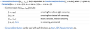
- CensoredDistribution[{xmin,xmax},dist] 等价于 TransformedDistribution[f,xdist],其中 f 由 Piecewise[{{xmin,x<=xmin},{x,xmin<x<xmax},{xmax,x>=xmax}}] 给出.
- {xmin,xmax} 的常见情形包括:
-
{-∞,xmax} 从上端删截,右删截 {xmin,∞} 从下端删截,左删截 {xmin,xmax} 双面删截,区间删截 {-∞,∞},None 无删截 - CensoredDistribution 可与 Mean、CDF、RandomVariate 等函数联合使用.
背景
- CensoredDistribution[{xmin,xmax},dist] 表示一个从区间

内所有
的单变量分布中提取的对数据建模的统计分布,并且对于
总等于
(相应的,对于
总等于
). 术语未删截、左删截、右删截和双删截分别描述 {xmin,xmax} 是 {-∞,∞}、{xmin,∞}、{-∞,xmax} 和 {xmin,xmax} 形式的单变量删截,其中单变量 dist 可以是连续的(如 NormalDistribution、 GammaDistribution 或 BetaDistribution)或离散的(如 PoissonDistribution、 BinomialDistribution 或 BernoulliDistribution)并可以(分别通过 TransformedDistribution、 CensoredDistribution 和 TruncatedDistribution)作为已知分布的变形、删截或截断定义. - 类似地,多变量的 CensoredDistribution[{{
,
},{
,
},… ,{
,
}},dist] 表示从多变量分布 dist 中提取的向量
的分布,其中第
个成分
位于区间
中. 正如单变量的情况,多变量 dist 可以使连续的(如 MultinormalDistribution)或离散的( MultivariateHypergeometricDistribution),也可以(分别通过 CopulaDistribution 和 ProductDistribution)作为一只分布的耦合或乘积定义. - 当对只知道部分数值的数据(即那些只含有部分观测或精度受限的数据的数据集)进行建模时可用删截分布,而对含有删截值的数据集的分析可以追溯到18世纪 Daniel Bernoulli 对天花的研究. 这样的数据在医药和心理学等领域中是比较普遍的,在不时需要未发现世纪故障时做出失效预测的可靠性和制造业中也相对普遍. 删截分布也是生存分析中的常用工具,以及为分析这样的数据集而存在的各种专业统计工具(如删失回归).
- 根据定义, CensoredDistribution[{xmin,xmax},dist] 等价于 TransformedDistribution[f,xdist],其中 f 由 Piecewise[{{xmin,x<=xmin},{x,xmin<x<xmax},{xmax,x>=xmax}}] 给出. CensoredDistribution 常与 TruncatedDistribution 混淆,但这两者有本质上的区别,删截将概率置于删截区间最后,而截尾将概率分布在截尾区间上.
范例
打开所有单元 关闭所有单元基本范例 (2)
𝒟 = CensoredDistribution[{5, ∞}, 𝒹 = BinomialDistribution[10, .6]];DiscretePlot[{PDF[𝒹, x], PDF[𝒟, x]}//Evaluate, {x, 0, 12}, ExtentSize -> 1 / 2, PlotLegends -> {"𝒹", "𝒟"}]𝒟 = CensoredDistribution[{-∞, 2}, 𝒩 = NormalDistribution[1, 2]];Plot[CDF[First[#], x]//Evaluate, {x, -4, 7}, Exclusions -> None, Filling -> Axis, PlotLabel -> Last[#]]& /@ {{𝒟, "𝒟"}, {𝒩, "𝒩"}}范围 (26)
基本用途 (9)
LeftCensored𝒟 = CensoredDistribution[{5, ∞}, PoissonDistribution[7]];
RightCensored𝒟 = CensoredDistribution[{-∞, 9}, PoissonDistribution[7]];
DoubleCensored𝒟 = CensoredDistribution[{5, 9}, PoissonDistribution[7]];Table[DiscretePlot[{PDF[m, x], PDF[PoissonDistribution[7], x]}//Evaluate, {x, 0, 13}, ExtentSize -> 0.5], {m, {LeftCensored𝒟, RightCensored𝒟, DoubleCensored𝒟}}]LeftCensored𝒟 = CensoredDistribution[{-1, ∞}, NormalDistribution[]];
RightCensored𝒟 = CensoredDistribution[{-∞, 1}, NormalDistribution[]];
DoubleCensored𝒟 = CensoredDistribution[{-1, 1}, NormalDistribution[]];Table[Plot[{CDF[m, x], CDF[NormalDistribution[], x]}, {x, -3, 3}, Filling -> Axis, Exclusions -> None], {m, {LeftCensored𝒟, RightCensored𝒟, DoubleCensored𝒟}}]𝒟 = CensoredDistribution[{0, 9}, 𝒹 = BinomialDistribution[12, .7]];DiscretePlot[{PDF[𝒹, x], PDF[𝒟, x]}, {x, 3, 13}, ExtentSize -> 1 / 2, PlotLegends -> {"𝒹", "𝒟"}]PDF[𝒟, 9]Probability[x ≥ 9, x𝒹]𝒟 = CensoredDistribution[{-1, ∞}, NormalDistribution[]];CDF[𝒟, x]Show[Histogram[RandomVariate[𝒟, 10 ^ 3], {-3, 3, .2}, "PDF"], Plot[PDF[NormalDistribution[], x], {x, -3, 3}, PlotStyle -> Thick]]𝒟1 = CensoredDistribution[{2, 2}, BinomialDistribution[3, .4]];PDF[𝒟1, x]𝒟2 = CensoredDistribution[{2, 2}, ParetoDistribution[1, 1 / 3]];CDF[𝒟2, x]𝒟 = CensoredDistribution[{{1 / 3, 1 / 2}, {2 / 5, 4 / 5}}, DirichletDistribution[{1, 3, 2}]];NExpectation[x ^ 2 + y, {x, y}𝒟]𝒟 = CensoredDistribution[{{2, 10}, {4, 12}, {3, 19}}, MultinomialDistribution[20, {1 / 3, 1 / 2, 1 / 6}]];Mean[𝒟]//Ndata = RandomVariate[𝒟, 10 ^ 4];Mean[data]//N𝒟 = CensoredDistribution[{1.2, 2}, 𝒹 = TriangularDistribution[{0, 4}]];Plot[{CDF[𝒹, x], CDF[𝒟, x]}//Evaluate, {x, 0, 5 / 2}, PlotStyle -> {Automatic, Thick}, Filling -> {2 -> Axis}, Exclusions -> None, PlotLegends -> {"𝒹", "𝒟"}]{Mean[𝒟], Variance[𝒟]}Moment 具有符号式阶数的解析式:
Moment[𝒟, r]data = RandomVariate[CensoredDistribution[{2, 7}, PoissonDistribution[5]], 10 ^ 2];edist = EstimatedDistribution[data, CensoredDistribution[{a, b}, PoissonDistribution[5]]]参数分布 (5)
𝒟 = CensoredDistribution[{0, 1 / 2}, BetaDistribution[2, 3]];CDF[𝒟, x]绘制随机样本的直方图. 尖峰对应于 PDF 的 DiracDelta 部分:
Show[Histogram[RandomVariate[𝒟, 10 ^ 3], Automatic, "PDF"], Plot[PDF[𝒟, x]//Evaluate, {x, 0, 1}, PlotStyle -> Thick, Exclusions -> None]]定义一个删截的 GeometricDistribution:
𝒟 = CensoredDistribution[{2, 5}, 𝒹 = GeometricDistribution[.2]];DiscretePlot[{PDF[𝒹, x], PDF[𝒟, x]}//Evaluate, {x, 0, 10}, ExtentSize -> 1 / 2, PlotLegends -> {"𝒹", "𝒟"}]PDF[𝒟, x]{Probability[x ≤ 2, x𝒹], PDF[𝒟, 2]}{Probability[x ≥ 5, x𝒹], PDF[𝒟, 5]}定义一个双删截 GammaDistribution:
𝒟 = CensoredDistribution[{2, 4}, GammaDistribution[2, 1]];CharacteristicFunction[𝒟, t]//FullSimplifyMomentGeneratingFunction[𝒟, t]//FullSimplifyCumulantGeneratingFunction[𝒟, t]//FullSimplifyFactorialMomentGeneratingFunction[𝒟, t]//FullSimplify定义一个右删截 PoissonDistribution:
𝒟 = CensoredDistribution[{-∞, 7}, 𝒫 = PoissonDistribution[5]];比较 HazardFunction:
DiscretePlot[{HazardFunction[𝒫, x], HazardFunction[𝒟, x]}, {x, 0, 9}, PlotRange -> All, ExtentSize -> 1 / 2]定义一个二维删截 DirichletDistribution:
𝒟 = CensoredDistribution[{{1 / 3, 1 / 2}, {1 / 3, 3 / 5}}, 𝒹 = DirichletDistribution[{3, 2, 4}]];Plot3D[CDF[#, {x, y}]//Evaluate, {x, -1 / 10, 3 / 4}, {y, -1 / 10, 4 / 5}, PlotRange -> All, AxesLabel -> Automatic, Exclusions -> None]& /@ {𝒹, 𝒟}Mean[𝒟]Variance[𝒟]NProbability[2 / 5 < x < 23 / 50 && y > 2 / 5, {x, y}𝒟]NExpectation[x ^ 3 + y ^ 3, {x, y}𝒟]非参数分布 (3)
定义一个删截的 EmpiricalDistribution:
ed = EmpiricalDistribution[RandomVariate[WeibullDistribution[2, 3], 15]];
𝒟 = CensoredDistribution[{0, 2}, ed];Plot[{CDF[ed, x], CDF[𝒟, x]}, {x, 0, 6}, Filling -> Axis, PlotStyle -> {Automatic, Thick}, Exclusions -> None, PlotLegends -> {"ed", "𝒟"}]定义一个删截的 HistogramDistribution:
hd = HistogramDistribution[RandomVariate[PoissonDistribution[6], 10 ^ 3]];
𝒟 = CensoredDistribution[{0, 6}, hd];Plot[{CDF[hd, x], CDF[𝒟, x]}, {x, 0, 12}, Filling -> Axis, Exclusions -> None, PlotStyle -> {Automatic, Thick}, PlotLegends -> {"hd", "𝒟"}]定义一个删截的 SmoothKernelDistribution:
skd = SmoothKernelDistribution[RandomVariate[LaplaceDistribution[0, 2], 10 ^ 3]];
𝒟 = CensoredDistribution[{-1, 1}, skd];Plot[{CDF[skd, x], CDF[𝒟, x]}, {x, -3, 3}, Filling -> Axis, PlotStyle -> {Automatic, Thick}, Exclusions -> None, PlotLegends -> {"skd", "𝒟"}]导出分布 (9)
定义一个删截 ParameterMixtureDistribution:
ℳ = ParameterMixtureDistribution[GammaDistribution[1 / 2, β], βUniformDistribution[{1, 2}]];
𝒟 = CensoredDistribution[{0, 1}, ℳ];CDF[𝒟, x]Plot[CDF[First[#], x]//Evaluate, {x, 0, 2}, Filling -> Axis, Exclusions -> None, PlotLabel -> Last[#]]& /@ {{ℳ, "ℳ"}, {𝒟, "𝒟"}}定义一个删截 MixtureDistribution:
ℳ = MixtureDistribution[{1, 2}, {NormalDistribution[-1, 3], NormalDistribution[1, 2]}];
𝒟 = CensoredDistribution[{-2, 2}, ℳ];CDF[𝒟, x]Plot[Evaluate[CDF[First[#], x]], {x, -3, 3}, Filling -> Axis, Exclusions -> None, PlotLabel -> Last[#]]& /@ {{ℳ, "ℳ"}, {𝒟, "𝒟"}}定义一个删截 OrderDistribution:
𝒫 = OrderDistribution[{BinomialDistribution[10, 0.6], 4}, 1];
𝒟 = CensoredDistribution[{4, ∞}, 𝒫];DiscretePlot[{PDF[𝒫, x], PDF[𝒟, x]}, {x, 0, 10}, ExtentSize -> 1 / 2, PlotLegends -> {"𝒫", "𝒟"}]{Mean[𝒟], Mean[𝒫]}定义一个删截 CensoredDistribution:
𝒞 = CensoredDistribution[{-∞, 9}, 𝒫 = PoissonDistribution[7]];
𝒟 = CensoredDistribution[{6, ∞}, 𝒞];DiscretePlot[Evaluate[PDF[First[#], x]], {x, 0, 15}, ExtentSize -> 1 / 2, PlotLabel -> Last[#]]& /@ {{𝒫, "𝒫"}, {𝒞, "𝒞"}, {𝒟, "𝒟"}}PDF[𝒟, x]PDF[CensoredDistribution[{6, 9}, PoissonDistribution[7]], x]% - %%定义一个删截 TruncatedDistribution:
𝒯 = TruncatedDistribution[{-∞, 1}, 𝒩 = NormalDistribution[0, 2]];
𝒟 = CensoredDistribution[{-1, ∞}, 𝒯];Plot[Evaluate[CDF[First[#], x]], {x, -3, 3}, Filling -> Axis, Exclusions -> None, PlotLabel -> Last[#]]& /@ {{𝒩, "𝒩"}, {𝒯, "𝒯"}, {𝒟, "𝒟"}}定义一个删截 TransformedDistribution:
𝒯 = TransformedDistribution[u + 1, uBenfordDistribution[10]];
𝒟 = CensoredDistribution[{3, 6}, 𝒯];CDF[𝒟, x]定义一个删截 MarginalDistribution:
ℳ = MarginalDistribution[NegativeMultinomialDistribution[3, {1 / 3, 1 / 3, 1 / 6}], 1];
𝒟 = CensoredDistribution[{3, 10}, ℳ];pdf = PDF[𝒟, x]DiscretePlot[{PDF[ℳ, x], pdf}, {x, 0, 15}, ExtentSize -> 1 / 2, PlotLegends -> {"ℳ", "𝒟"}]定义一个删截 ProductDistribution:
𝒫 = ProductDistribution[PoissonDistribution[8], PoissonDistribution[9]];
𝒟 = CensoredDistribution[{{-∞, 12}, {5, ∞}}, 𝒫];Histogram3D[RandomVariate[𝒟, 10 ^ 4], 20, "PDF"]QuantityDistribution 的删截估值为 QuantityDistribution:
𝒟 = CensoredDistribution[{-∞, Quantity[75, "Miles"/"Hours"]}, QuantityDistribution[NormalDistribution[70, 8], "mph"]]Mean[𝒟]//N应用 (4)
一家保险公司在留用水平
处购买再保险. 假定索赔服从对数正态分布,求保险公司支付额随机变量的矩:
Refine[Moment[CensoredDistribution[{0, M}, LogNormalDistribution[μ, σ]], n], M > 0 && σ > 0]Refine[Moment[CensoredDistribution[{M, Infinity}, LogNormalDistribution[μ, σ]], n], M > 0 && σ > 0]一个组件的生命期服从 RayleighDistribution. 使用
小时时间,对组件进行检测,如果在这段时间内组件没有失效,那么假定这个组件的生命期恰好是
小时. 求满足至少有 5% 的被检测组件的生命期长于
的条件下,检测的时间长度:
component𝒟 = RayleighDistribution[Quantity[3, "Hours"]]Solve[CDF[component𝒟, n] == 95 / 100, n]N[%]test𝒟 = CensoredDistribution[{Quantity[0, "Hours"], Quantity[7.35, "Hours"]}, component𝒟];Plot[{CDF[component𝒟, Quantity[x, "Hours"]], CDF[test𝒟, Quantity[x, "Hours"]]}, {x, 0, 10}, Filling -> 1 -> {2}, Epilog -> {Dashed, Line[{{7.35, 0}, {7.35, 1}}]}, PlotLegends -> {"component𝒟", "test𝒟"}, AxesLabel -> {"h"}]Mean /@ {component𝒟, test𝒟}//N一名高尔夫初学者要使球进入一个四杆洞所需的击球次数服从均值为 8 的一个 PoissonDistribution 分布. 假定在这个高尔夫球场上,在第10次击球后,这名选手就把球捡起来,求在一个四杆洞中球入洞次数的分布:
𝒟 = TransformedDistribution[u + 1, uCensoredDistribution[{0, 9}, PoissonDistribution[8]]];DiscretePlot[Evaluate[PDF[𝒟, x]], {x, 0, 11}, ExtentSize -> 1 / 2]PDF[𝒟, x]Mean[𝒟]//NNProbability[x > 4, x𝒟]美国成年男性的体重服从均值为 191 磅、标准差为 70 磅的正态分布. 假定每个浴室磅秤的上限为 300 磅,求当使用普通浴室磅秤测量时得到的体重分布:
𝒟 = CensoredDistribution[{Quantity[0, "Pounds"], Quantity[300, "Pounds"]}, 𝒹 = NormalDistribution[Quantity[191, "Pounds"], Quantity[70, "Pounds"]]];Plot[Evaluate[CDF[𝒟, Quantity[x, "Pounds"]]], {x, 0, 350}, Filling -> Axis, Exclusions -> None, AxesLabel -> {"lbs"}]Histogram[RandomVariate[𝒟, 10 ^ 5], Automatic, "PDF", AxesLabel -> Automatic]Mean[𝒟]//NNProbability[x ≥ Quantity[200, "Pounds"], x𝒟]Probability[x ≥ Quantity[300, "Pounds"], x𝒟]//NProbability[x ≥ Quantity[300, "Pounds"], x𝒹]//N属性和关系 (4)
CensoredDistribution 是 TransformedDistribution 的一种特殊情况:
𝒟1 = CensoredDistribution[{2, 3}, NormalDistribution[]];
𝒟2 = TransformedDistribution[Piecewise[{{2, u ≤ 2}, {u, 2 ≤ u ≤ 3}, {3, u > 3}}], uNormalDistribution[]];CDF[𝒟1, x]CDF[𝒟2, x]% - %%//FullSimplify𝒞 = CensoredDistribution[{4, 9}, 𝒫 = PoissonDistribution[7]];
𝒯 = TruncatedDistribution[{4, 9}, 𝒫];DiscretePlot[{PDF[𝒫, x], PDF[𝒞, x]}, {x, 0, 12}, ExtentSize -> 1 / 2, PlotLegends -> {"𝒫", "𝒞"}]DiscretePlot[{PDF[𝒫, x], PDF[𝒯, x]}, {x, 0, 12}, ExtentSize -> 1 / 2, PlotLegends -> {"𝒫", "𝒯"}]𝒞 = CensoredDistribution[{1 / 2, ∞}, 𝒩 = NormalDistribution[0, 1 / 2]];
𝒯 = TruncatedDistribution[{1 / 2, ∞}, 𝒩];Plot[{CDF[𝒩, x], CDF[𝒞, x]}, {x, -2, 3}, Filling -> Axis, PlotLegends -> {"𝒩", "𝒞"}]Plot[{CDF[𝒩, x], CDF[𝒯, x]}, {x, -2, 3}, Filling -> Axis, PlotLegends -> {"𝒩", "𝒯"}]一个连续分布的删截可能会导致一个既不连续又不离散的混合分布:
cont𝒟 = LogisticDistribution[];
cens𝒟 = CensoredDistribution[{-1, 1}, cont𝒟]该混合型删截分布的 CDF 在删截点不连续:
cdf = CDF[cens𝒟, x]ticks = {{-1, -0.5, 0, 0.5, 1}, {0, {CDF[cont𝒟, -1], HoldForm[F[-1 + ϵ]]}, 0.5, {CDF[cont𝒟, 1], HoldForm[F[1 - ϵ]]}, 1}};
Plot[{cdf, Style[CDF[cont𝒟, x], DotDashed]}, {x, -1.75, 1.75}, Ticks -> ticks, ExclusionsStyle -> {Directive[Dotted, Red], PointSize[Medium]}, PlotLegends -> {"censored 𝒟", "underlying continuous 𝒟"}]删截分布的概率密度函数没有定义, PDF 返回未估值:
PDF[cens𝒟, x]D[cdf, x]NIntegrate[D[cdf, x], {x, -∞, ∞}]Table[Labeled[Histogram[RandomVariate[cens𝒟, 10 ^ k], "Scott", "PDF", ImageSize -> Small], Row[{Text@"Sample size", ":", HoldForm[10] ^ k//TraditionalForm}]], {k, {3, 6}}]Table[Labeled[Histogram[RandomVariate[cont𝒟, 10 ^ k], "Scott", "PDF", ImageSize -> Small], Row[{Text@"Sample size", ":", HoldForm[10] ^ k//TraditionalForm}]], {k, {3, 6}}]可能存在的问题 (1)
cont𝒟 = NormalDistribution[];
cens𝒟 = CensoredDistribution[{-1, 1}, cont𝒟]PDF[cens𝒟, x]{Mean[cens𝒟], Variance[cens𝒟], Skewness[cens𝒟], Kurtosis[cens𝒟]}sample = RandomVariate[cens𝒟, 10 ^ 4];EstimatedDistribution[sample, CensoredDistribution[{min, max}, NormalDistribution[μ, σ]]]ProbabilityDistribution[{CDF, CDF[cens𝒟, x]}, {x, -Infinity, Infinity}]//FullSimplify相关指南
-
▪
- 用于可靠性分析中的分布 ▪
- 导出统计分布 ▪
- 有界域分布 ▪
- 随机变量
文本
Wolfram Research (2010),CensoredDistribution,Wolfram 语言函数,https://reference.wolfram.com/language/ref/CensoredDistribution.html (更新于 2016 年).
CMS
Wolfram 语言. 2010. "CensoredDistribution." Wolfram 语言与系统参考资料中心. Wolfram Research. 最新版本 2016. https://reference.wolfram.com/language/ref/CensoredDistribution.html.
APA
Wolfram 语言. (2010). CensoredDistribution. Wolfram 语言与系统参考资料中心. 追溯自 https://reference.wolfram.com/language/ref/CensoredDistribution.html 年
BibTeX
@misc{reference.wolfram_2026_censoreddistribution, author="Wolfram Research", title="{CensoredDistribution}", year="2016", howpublished="\url{https://reference.wolfram.com/language/ref/CensoredDistribution.html}", note=[Accessed: 18-August-2026]}
BibLaTeX
@online{reference.wolfram_2026_censoreddistribution, organization={Wolfram Research}, title={CensoredDistribution}, year={2016}, url={https://reference.wolfram.com/language/ref/CensoredDistribution.html}, note=[Accessed: 18-August-2026]}