



ComplexContourPlot
ComplexContourPlot[f,{z,zmin,zmax}]
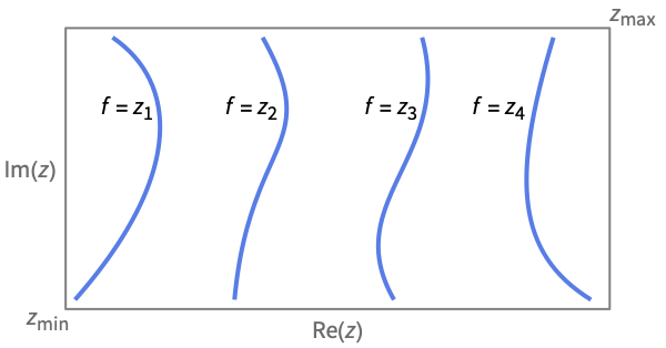
生成 f 作为 z 的函数的填充等值线图.
ComplexContourPlot[{f1,f2,…},{z,zmin,zmax}]
生成 f1、f2、… 的等值线.
ComplexContourPlot[f==g,{z,zmin,zmax}]
绘制 f=g 的等值线.
ComplexContourPlot[{f1==g1,f2==g2,…},{z,zmin,zmax}]
绘制 f1g1、f2=g2、… 的等值线.
更多信息和选项
- 在 f 值不为实数的位置,会留下孔,可看到等值线图的背景. 函数 f 和 g 通常会涉及如 Re、Im、Abs 和 Arg 等这样的函数,从复数中提取实部以进行比较.
- ComplexContourPlot[f,{z,n}] 等价于 ComplexContourPlot[f,{z,-n-n I,n+n I}].
- ComplexContourPlot 将变量 z 视为局部变量,相当于使用 Block.
- ComplexContourPlot 具有属性 HoldAll,在对 z 赋值后才计算 fi 和 gi. 某些情况下,先用 Evaluate 对 f 和 g 进行符号式计算效率更高.
- ComplexContourPlot 和 Graphics 有相同的选项,不同之处和更多选项如下所示: [所有选项的列表]
- PlotLegends 的常见设置有:
-
None 没有图例 Automatic 自动确定图例 Placed[lspec,…] 指定图例的放置 - 当采用默认设置 ContourShading->Automatic 时,对 ComplexContourPlot[f,…] 使用色调处理,但不对 ComplexContourPlot[f=g,…] 或 ComplexContourPlot[{f1,f2,…},…] 使用色调处理.
- ComplexContourPlot[{f1==g1,f2==g2,…},…] 叠加显示与等式 fi==gi 关联的所有等值线.
- 在确定如何为等值线之间的区域进行着色时,ComplexContourPlot 首先查看 ContourShading 的显式设置,然后 查看 ColorFunction 的设置.
- 在绘制多个函数的等值线 ComplexContourPlot[{f1,f2,…},…] 时,等值线指定列表 Contours{spec1,spec2,…} 将对每个 fi 使用相应的 speci.
- ColorData["DefaultPlotColors"] 给出 ContourStyle 使用的默认颜色序列.
- ComplexContourPlot 首先在由 PlotPoints 指定的等间隔采样点组成的网格上计算 f. 然后使用一种自适应算法进行至多 MaxRecursion 次子划分,来产生平滑的等值线.
- 应该认识到由于使用的采样点数量有限,ComplexContourPlot 可能会丢失函数的部分特征. 为确保结果正确,可以尝试增大 PlotPoints 和 MaxRecursion 的设置.
- 对于 PerformanceGoal 的某些设置,其它特定选项设置可能会被屏蔽.
- 为 MeshFunctions 和 RegionFunction 中的函数提供的参数为 z、f.
- 只为 ColorFunction 提供一个参数,默认情况下为相邻等值线的缩放过的 f 值的平均值.
- 当采用默认设置 Exclusions->Automatic 和 ExclusionsStyle->None 时,ComplexContourPlot 在它检测到的所有不连续曲线处打破其采样的连续性. 仅当不连续性跳离特定等值线时,该不连续性才立即可见.
- ScalingFunctions 的可能设置包括:
-
sf 缩放 f 值 {sRe,sIm} 缩放实轴和虚轴 {sRe,sIm,sf} 缩放实轴、虚轴及 f 值
所有选项的列表
范例
打开所有单元 关闭所有单元基本范例 (4)
ComplexContourPlot[Abs[z], {z, -3 - 3I, 3 + 3I}]ComplexContourPlot[Re[z] == Im[1 / z], {z, 2}]ComplexContourPlot[{Re[z], Im[1 / z]}, {z, 2}]ComplexContourPlot[{Abs[z] == Re[z] + 1, Abs[z] == Re[z] + 2, Abs[z] == Re[z] + 3}, {z, -3 - 3I, 3 + 3I}, PlotLegends -> "Expressions"]范围 (18)
采样 (6)
ComplexContourPlot[Abs[z^2 + 1], {z, 0, 2 + 2I}, Mesh -> All]ComplexContourPlot[Abs[1 / z], {z, -3 - 3I, 3 + 3I}]用 PlotRange 选取感兴趣的区域:
ComplexContourPlot[Abs[1 / z], {z, -3 - 3I, 3 + 3I}, PlotRange -> {0.2, 5}]用 PlotPoints 和 MaxRecursion 控制自适应采样:
Table[ComplexContourPlot[Abs[Sin[z^1 / 2] + 1], {z, 0, 2 + 2I}, PlotPoints -> pp, MaxRecursion -> mr], {mr, {0, 2}}, {pp, {5, 15}}]用 RegionFunction 将曲面限制在不等式给定的区域上:
ComplexContourPlot[Re[ArcSin[z]], {z, -3 - 3I, 3 + 3I}, RegionFunction -> Function[{z, f}, Abs[z] < 3]]用 Exclusions 控制有断点时是否及在何处切割:
{ComplexContourPlot[Arg[ArcSin[z^2]], {z, -3 - 3I, 3 + 3I}],
	ComplexContourPlot[Arg[ArcSin[z^2]], {z, -3 - 3I, 3 + 3I}, Exclusions -> None]}
添加标签和图例 (6)
ComplexContourPlot[Re[Sqrt[z]], {z, -3 - 3I, 3 + 3I}, FrameLabel -> {Re[z], Im[z]}, PlotLabel -> Re[Sqrt[z]]]ComplexContourPlot[Re[Sqrt[z]] == 1, {z, -3 - 3I, 3 + 3I}, FrameLabel -> {Re[z], Im[z]}, PlotLabel -> Re[Sqrt[z]] == 1]ComplexContourPlot[Re[Sqrt[z]], {z, -3 - 3I, 3 + 3I}, ContourLabels -> True]ComplexContourPlot[Re[Sqrt[z]], {z, -3 - 3I, 3 + 3I}, PlotLegends -> Automatic]ComplexContourPlot[ReIm[Sqrt[z]], {z, -3 - 3I, 3 + 3I}, PlotLegends -> "Expressions"]ComplexContourPlot[ReIm[Sqrt[z]], {z, -3 - 3I, 3 + 3I}, PlotLegends -> Automatic]ComplexContourPlot[{Re[z^2] == 1, Im[z^2] == 1}, {z, -3 - 3I, 3 + 3I}, PlotLegends -> "Expressions"]演示 (6)
ComplexContourPlot[Re[Sqrt[z]], {z, -3 - 3I, 3 + 3I}, ColorFunction -> "Rainbow"]ComplexContourPlot[Re[z^2], {z, -3 - 3I, 3 + 3I}, ContourShading -> Hue /@ Range[0, 1, 0.1]]ComplexContourPlot[Re[z^2], {z, -3 - 3I, 3 + 3I}, ContourStyle -> {Red, Directive[Red, Dashed]}]ComplexContourPlot[{Re[z^2] == 1, Im[z^2] == 1}, {z, -3 - 3I, 3 + 3I}, ContourStyle -> {Green, Dashed}]ComplexContourPlot[Re[z^2], {z, -3 - 3I, 3 + 3I}, Mesh -> 10, MeshFunctions -> {Re[#1]&, Im[#1]&}]ComplexContourPlot[Re[z^2], {z, -3 - 3I, 3 + 3I}, PlotTheme -> "Scientific"]选项 (138)
AspectRatio (4)
默认情况下,AspectRatio 使用相等的宽和高:
ComplexContourPlot[Abs[z^2 - 2], {z, -4 - 2I, 4 + 2I}]ComplexContourPlot[Abs[z^2 - 2], {z, -4 - 2I, 4 + 2I}, AspectRatio -> 1 / 2]AspectRatioAutomatic 根据绘图范围确定比率:
ComplexContourPlot[Abs[z^2 - 2], {z, -4 - 2I, 4 + 2I}, AspectRatio -> Automatic]AspectRatioFull 调整高度和宽度以紧密贴合其他构造:
plot = ComplexContourPlot[Abs[z^2 - 2], {z, -4 - 2I, 4 + 2I}, AspectRatio -> Full];{Framed[Pane[plot, {240, 200}]], Framed[Pane[plot, {230, 230}]]}Axes (4)
默认情况下,ComplexContourPlot 使用边框而非轴:
ComplexContourPlot[Abs[Sin[z^1 / 2 - 3]], {z, -4 - 4I, 4 + 4I}]ComplexContourPlot[Abs[Sin[z^1 / 2 - 3]], {z, -4 - 4I, 4 + 4I}, Frame -> False, Axes -> True]使用 AxesOrigin 可指定轴相交处:
ComplexContourPlot[Abs[Sin[z^1 / 2 - 3]], {z, -4 - 4I, 4 + 4I}, Frame -> False, Axes -> True, AxesOrigin -> {0, 0}]{ComplexContourPlot[Abs[Sin[z^1 / 2 - 3]], {z, -4 - 4I, 4 + 4I}, Frame -> False, Axes -> {True, False}], ComplexContourPlot[Abs[Sin[z^1 / 2 - 3]], {z, -4 - 4I, 4 + 4I}, Frame -> False, Axes -> {False, True}]}AxesLabel (3)
ComplexContourPlot[Abs[Sin[z^1 / 2 - 3]], {z, -4 - 4I, 4 + 4I}, Frame -> False, Axes -> True]
ComplexContourPlot[Abs[Sin[z^1 / 2 - 3]], {z, -4 - 4I, 4 + 4I}, Frame -> False, Axes -> True, AxesLabel -> Y]ComplexContourPlot[Abs[Sin[z^1 / 2 - 3]], {z, -4 - 4I, 4 + 4I}, Frame -> False, Axes -> True, AxesLabel -> {"X", "Y"}]AxesOrigin (2)
AxesStyle (4)
ComplexContourPlot[Abs[Sin[z^1 / 2 - 3]], {z, -4 - 4I, 4 + 4I}, Frame -> False, Axes -> True, AxesStyle -> Red]ComplexContourPlot[Abs[Sin[z^1 / 2 - 3]], {z, -4 - 4I, 4 + 4I}, Frame -> False, Axes -> True, AxesStyle -> {{Thick, Red}, {Thick, Blue}}]ComplexContourPlot[Abs[Sin[z^1 / 2 - 3]], {z, -4 - 4I, 4 + 4I}, Frame -> False, Axes -> True, AxesStyle -> Green, TicksStyle -> Black]ComplexContourPlot[Abs[Sin[z^1 / 2 - 3]], {z, -4 - 4I, 4 + 4I}, Frame -> False, Axes -> True, AxesStyle -> Green, LabelStyle -> Black]BoundaryStyle (3)
ComplexContourPlot[Abs[Sin[z^1 / 2 - 3]], {z, -4 - 4I, 4 + 4I}, BoundaryStyle -> Red]BoundaryStyle 也适用于由 RegionFunction 切割出的洞,但不适用于 Exclusions 造成的切割:
ComplexContourPlot[Abs[Sin[z^1 / 2 - 3]], {z, -4 - 4I, 4 + 4I}, BoundaryStyle -> Red, RegionFunction -> Function[{z, f}, Abs[z] > 2]]用 ExclusionsStyle 替代:
ComplexContourPlot[Abs[Sin[z^1 / 2 - 3]], {z, -4 - 4I, 4 + 4I}, ExclusionsStyle -> Red]ClippingStyle (4)
ComplexContourPlot[Re[Exp[I z^2]], {z, -3 - 3I, 3 + 3I}, ClippingStyle -> Automatic]ComplexContourPlot[Re[Exp[I z^2]], {z, -3 - 3I, 3 + 3I}, ClippingStyle -> None]ComplexContourPlot[Re[Exp[I z^2]], {z, -3 - 3I, 3 + 3I}, ClippingStyle -> Pink]如果是超过范围设置被剪切,使用绿色,如果小于范围设置被剪切,使用粉红色:
ComplexContourPlot[Re[Exp[I z^2]], {z, -3 - 3I, 3 + 3I}, ClippingStyle -> {Pink, Green}]ColorFunction (3)
ComplexContourPlot[Abs[Sin[z^1 / 2 - 3]], {z, -4 - 4I, 4 + 4I}, ColorFunction -> Hue]ComplexContourPlot[Abs[Sin[z^1 / 2 - 3]], {z, -4 - 4I, 4 + 4I}, ColorFunction -> "WatermelonColors"]
ComplexContourPlot[Abs[Sin[z^1 / 2 - 3]], {z, -4 - 4I, 4 + 4I}, ColorFunction -> (If[#1 > 1, Red, White]&), ColorFunctionScaling -> False]ColorFunctionScaling (1)
ColorFunction 可以使用缩放过的或未经缩放的坐标:
Table[ComplexContourPlot[Abs[z], {z, -2 - 2I, 2 + 2I}, Contours -> 20, ColorFunction -> Hue, ColorFunctionScaling -> cf], {cf, {True, False}}]ContourLabels (2)
Contours (9)
ComplexContourPlot[Im[z^3 + 1], {z, -1 - 1I, 1 + 1I}, Contours -> 10]ComplexContourPlot[Im[z^3 + 1], {z, -1 - 1I, 1 + 1I}, Contours -> Automatic]ComplexContourPlot[Im[z^3 + 1], {z, -1 - 1I, 1 + 1I}, Contours -> {Automatic, 5}]ComplexContourPlot[Im[z^3 + 1], {z, -1 - 1I, 1 + 1I}, Contours -> {-0.5, 0, 0.5}]ComplexContourPlot[Im[z^3 + 1], {z, -1 - 1I, 1 + 1I}, Contours -> {{-0.5, Red}, {0, Green}, {0.5, Blue}}]ComplexContourPlot[Im[z^3 + 1], {z, -1 - 1I, 1 + 1I}, Contours -> Function[{min, max}, Range[min, max, 0.1]]]ComplexContourPlot[Im[z^3 + 1], {z, -1 - 1I, 1 + 1I}, Contours -> Function[{min, max}, Rescale[{0.4, 0.8}, {0, 1}, {min, max}]]]ComplexContourPlot[ReIm[z^3 + 1], {z, -1 - 1I, 1 + 1I}, Contours -> {5, 10}]ComplexContourPlot[ReIm[z^3 + 1], {z, -1 - 1I, 1 + 1I}, Contours -> {Range[0, 1, 0.2], Range[0, 2, 0.1]}]ContourShading (5)
如果采用自动色调设置,则在数值较小处颜色较深,在数值较大处颜色较浅:
ComplexContourPlot[Im[z^3 + 1], {z, -1 - 1I, 1 + 1I}, ContourShading -> Automatic]用 None 只显示等值线:
ComplexContourPlot[Im[z^3 + 1], {z, -1 - 1I, 1 + 1I}, ContourShading -> None]ComplexContourPlot[ReIm[Sqrt[z]], {z, -3 - 3I, 3 + 3I}]ComplexContourPlot[Im[z^3 + 1], {z, -1 - 1I, 1 + 1I}, ContourShading -> Automatic, ColorFunction -> "Rainbow"]ComplexContourPlot[Im[z^3 + 1], {z, -1 - 1I, 1 + 1I}, Contours -> 3, ContourShading -> {Red, Orange, Yellow, White}]ContourStyle (7)
ComplexContourPlot[Im[z^3 + 1], {z, -1 - 1I, 1 + 1I}, ContourStyle -> Automatic]ComplexContourPlot[Im[z^3 + 1], {z, -1 - 1I, 1 + 1I}, ContourStyle -> Directive[Dashed, Opacity[1]]]用 None 隐去等值线:
ComplexContourPlot[Im[z^3 + 1], {z, -1 - 1I, 1 + 1I}, ContourStyle -> None]ContourStyleNone 等价于 ContourLinesFalse:
ComplexContourPlot[Im[z^3 + 1], {z, -1 - 1I, 1 + 1I}, ContourLines -> False, ContourStyle -> Black]ComplexContourPlot[Im[z^3 + 1], {z, -1 - 1I, 1 + 1I}, ContourStyle -> {Red, Dashed}]ComplexContourPlot[{Abs[z^2 + 1], Abs[z^2 - 1]}, {z, -2 - 2I, 2 + 2I}, ContourStyle -> {Red, Blue}]ComplexContourPlot[{Abs[z^3 + 1] == 2, Abs[z^3 - 1] == 2}, {z, -2 - 2I, 2 + 2I}, ContourStyle -> {Red, Dashed}]ComplexContourPlot[{Abs[z^3 + 1] == 2, Abs[z^3 - 1] == 2}, {z, -2 - 2I, 2 + 2I}, ContourStyle -> Directive[Red, Dashed]]EvaluationMonitor (2)
显示 ContourPlot 在函数取样的位置:
ComplexListPlot[Reap[ComplexContourPlot[Arg[ArcTan[z]], {z, -2 - 2I, 2 + 2I}, EvaluationMonitor :> Sow[z]]][[-1, 1]], PlotStyle -> PointSize[Tiny]]Block[{k = 0}, ComplexContourPlot[Arg[ArcTan[z]], {z, -2 - 2I, 2 + 2I}, EvaluationMonitor :> k++];k]Exclusions (6)
ComplexContourPlot[Re[ArcCos[z^2]], {z, -3 - 3I, 3 + 3I}]ComplexContourPlot[Re[ArcCos[z^2]], {z, -3 - 3I, 3 + 3I}, Exclusions -> None]ComplexContourPlot[Re[ArcCos[z^2]], {z, -3 - 3I, 3 + 3I}, Exclusions -> Im[z] == 0]ComplexContourPlot[Re[ArcCos[z^2]], {z, -3 - 3I, 3 + 3I}, Exclusions -> {Im[z] == 0, Re[z] == 0}]ComplexContourPlot[Re[ArcCos[z^2]], {z, -3 - 3I, 3 + 3I}, Exclusions -> {{Im[z] == 0, Abs[Re[z]] > 1}, {Re[z] == 0, Abs[Im[z]] > 1}}]ComplexContourPlot[Re[ArcCos[z^2]], {z, -3 - 3I, 3 + 3I}, Exclusions -> {Automatic, Abs[z] == 1}]ExclusionsStyle (2)
Frame (4)
ComplexContourPlot 默认使用边框:
ComplexContourPlot[{Abs[z] == Re[z] + 1, Abs[z] == Re[z] + 2, Abs[z] == Re[z] + 3}, {z, -3 - 3 I, 3 + 3 I}]ComplexContourPlot[{Abs[z] == Re[z] + 1, Abs[z] == Re[z] + 2, Abs[z] == Re[z] + 3}, {z, -3 - 3 I, 3 + 3 I}, Frame -> False]ComplexContourPlot[{Abs[z] == Re[z] + 1, Abs[z] == Re[z] + 2, Abs[z] == Re[z] + 3}, {z, -3 - 3 I, 3 + 3 I}, Frame -> {{True, True}, {False, False}}]ComplexContourPlot[{Abs[z] == Re[z] + 1, Abs[z] == Re[z] + 2, Abs[z] == Re[z] + 3}, {z, -3 - 3 I, 3 + 3 I}, Frame -> {{True, False}, {True, False}}]FrameLabel (4)
ComplexContourPlot[{Abs[z] == Re[z] + 1, Abs[z] == Re[z] + 2, Abs[z] == Re[z] + 3}, {z, -3 - 3 I, 3 + 3 I}, FrameLabel -> {"label"}]ComplexContourPlot[{Abs[z] == Re[z] + 1, Abs[z] == Re[z] + 2, Abs[z] == Re[z] + 3}, {z, -3 - 3 I, 3 + 3 I}, FrameLabel -> Automatic]ComplexContourPlot[{Abs[z] == Re[z] + 1, Abs[z] == Re[z] + 2, Abs[z] == Re[z] + 3}, {z, -3 - 3 I, 3 + 3 I}, FrameLabel -> {{"left", "right"}, {"bottom", "top"}}]ComplexContourPlot[{Abs[z] == Re[z] + 1, Abs[z] == Re[z] + 2, Abs[z] == Re[z] + 3}, {z, -3 - 3 I, 3 + 3 I}, FrameLabel -> {{"left", "right"}, {"bottom", "top"}}, LabelStyle -> Directive[Bold, StandardGray]]FrameStyle (2)
ComplexContourPlot[{Abs[z] == Re[z] + 1, Abs[z] == Re[z] + 2, Abs[z] == Re[z] + 3}, {z, -3 - 3 I, 3 + 3 I}, FrameStyle -> Directive[StandardGray, Thick]]ComplexContourPlot[{Abs[z] == Re[z] + 1, Abs[z] == Re[z] + 2, Abs[z] == Re[z] + 3}, {z, -3 - 3 I, 3 + 3 I}, FrameStyle -> {{Directive[Green, Thick], Directive[Red]}, {Directive[Gray, Thick], Directive[Blue]}}]FrameTicks (9)
ComplexContourPlot[{Abs[z] == Re[z] + 1, Abs[z] == Re[z] + 2, Abs[z] == Re[z] + 3}, {z, -3 - 3 I, 3 + 3 I}]ComplexContourPlot[{Abs[z] == Re[z] + 1, Abs[z] == Re[z] + 2, Abs[z] == Re[z] + 3}, {z, -3 - 3 I, 3 + 3 I}, FrameTicks -> None]ComplexContourPlot[{Abs[z] == Re[z] + 1, Abs[z] == Re[z] + 2, Abs[z] == Re[z] + 3}, {z, -3 - 3 I, 3 + 3 I}, FrameTicks -> {{None, None}, {Automatic, None}}]ComplexContourPlot[{Abs[z] == Re[z] + 1, Abs[z] == Re[z] + 2, Abs[z] == Re[z] + 3}, {z, -3 - 3 I, 3 + 3 I}, FrameTicks -> Automatic]使用 All 可在所有边上添加刻度标签:
ComplexContourPlot[{Abs[z] == Re[z] + 1, Abs[z] == Re[z] + 2, Abs[z] == Re[z] + 3}, {z, -3 - 3 I, 3 + 3 I}, FrameTicks -> All]ComplexContourPlot[{Abs[z] == Re[z] + 1, Abs[z] == Re[z] + 2, Abs[z] == Re[z] + 3}, {z, -5 - 5 I, 5 + 5 I}, FrameTicks -> {{{1, 3, 5}, {1, 3, 5}}, {{1, 3, 4}, {1, 3, 4}}}]ComplexContourPlot[{Abs[z] == Re[z] + 1, Abs[z] == Re[z] + 2, Abs[z] == Re[z] + 3}, {z, -5 - 5 I, 5 + 5 I}, FrameTicks -> {{{{1, a}, {3, b}, {5, d}}, Automatic}, {{{1, a}, {3, b}, {4, c}}, Automatic}}]ComplexContourPlot[{Abs[z] == Re[z] + 1, Abs[z] == Re[z] + 2, Abs[z] == Re[z] + 3}, {z, -5 - 5 I, 5 + 5 I}, FrameTicks -> {{{{1, a, .37}, {3, b, .5}, {5, d, .75}}, Automatic}, {{{1, a, .13}, {3, b, .12}, {4, c, .2}}, Automatic}}]ComplexContourPlot[{Abs[z] == Re[z] + 1, Abs[z] == Re[z] + 2, Abs[z] == Re[z] + 3}, {z, -5 - 5 I, 5 + 5 I}, FrameTicks -> {{Automatic, Automatic}, {{{1, a, {.13, 0.05}}, {3, b, {.12, .1}}, {4, c, {.2, .2}}}, Automatic}}]ComplexContourPlot[{Abs[z] == Re[z] + 1, Abs[z] == Re[z] + 2, Abs[z] == Re[z] + 3}, {z, -5 - 5 I, 5 + 5 I}, FrameTicks -> {{{{1, a, .37, Directive[Red]}, {3, b, .5, Directive[Red, Thick, Dashed]}, {5, d, .75, Directive[Green, Thick, Dashed]}}, Automatic}, {Automatic, Automatic}}]minMeanMax[min_, max_] := {{min, min}, {(max + min) / 2, (max + min) / 2}, {max, max}}ComplexContourPlot[{Abs[z] == Re[z] + 1, Abs[z] == Re[z] + 2, Abs[z] == Re[z] + 3}, {z, -1 - 1 I, 5 + 5 I}, FrameTicks -> {{minMeanMax, None}, {minMeanMax, None}}, PlotRangePadding -> None]FrameTicksStyle (3)
ComplexContourPlot[{Abs[z] == Re[z] + 1, Abs[z] == Re[z] + 2, Abs[z] == Re[z] + 3}, {z, -3 - 3 I, 3 + 3 I}, FrameStyle -> Directive[Red]]ComplexContourPlot[{Abs[z] == Re[z] + 1, Abs[z] == Re[z] + 2, Abs[z] == Re[z] + 3}, {z, -3 - 3 I, 3 + 3 I}, FrameTicksStyle -> Directive[Blue, Thick]]ComplexContourPlot[{Abs[z] == Re[z] + 1, Abs[z] == Re[z] + 2, Abs[z] == Re[z] + 3}, {z, -3 - 3 I, 3 + 3 I}, FrameTicksStyle -> {{Directive[StandardGray, Thick], Blue}, {Red, Green}}]ImageSize (7)
使用有名称的尺寸如 Tiny、Small、Medium 和 Large:
{ComplexContourPlot[Abs[z^2 - 2], {z, -4 - 2I, 4 + 2I}, ImageSize -> Tiny], ComplexContourPlot[Abs[z^2 - 2], {z, -4 - 2I, 4 + 2I}, ImageSize -> Small]}{ComplexContourPlot[Abs[z^2 - 2], {z, -4 - 2I, 4 + 2I}, ImageSize -> 150], ComplexContourPlot[Abs[z^2 - 2], {z, -4 - 2I, 4 + 2I}, AspectRatio -> 1.5, ImageSize -> 150]}{ComplexContourPlot[Abs[z^2 - 2], {z, -4 - 2I, 4 + 2I}, ImageSize -> {Automatic, 150}], ComplexContourPlot[Abs[z^2 - 2], {z, -4 - 2I, 4 + 2I}, AspectRatio -> 2, ImageSize -> {Automatic, 150}]}{ComplexContourPlot[Abs[z^2 - 2], {z, -4 - 2I, 4 + 2I}, ImageSize -> UpTo[200]], ComplexContourPlot[Abs[z^2 - 2], {z, -4 - 2I, 4 + 2I}, AspectRatio -> 2, ImageSize -> UpTo[200]]}ComplexContourPlot[Abs[z^2 - 2], {z, -4 - 2I, 4 + 2I}, ImageSize -> {200, 300}, Background -> StandardBlue]设置 AspectRatioFull 将填充可用空间:
ComplexContourPlot[Abs[z^2 - 2], {z, -4 - 2I, 4 + 2I}, AspectRatio -> Full, ImageSize -> {200, 300}, Background -> StandardBlue]{ComplexContourPlot[Abs[z^2 - 2], {z, -4 - 2I, 4 + 2I}, ImageSize -> {UpTo[150], UpTo[100]}], ComplexContourPlot[Abs[z^2 - 2], {z, -4 - 2I, 4 + 2I}, AspectRatio -> 2, ImageSize -> {UpTo[150], UpTo[100]}]}Framed[Pane[ComplexContourPlot[Abs[z^2 - 2], {z, -4 - 2I, 4 + 2I}, ImageSize -> Full, Background -> StandardBlue], {200, 100}]]Framed[Pane[ComplexContourPlot[Abs[z^2 - 2], {z, -4 - 2I, 4 + 2I}, AspectRatio -> Full, ImageSize -> {Scaled[0.5], Scaled[0.5]}, Background -> StandardBlue], {200, 100}]]MaxRecursion (1)
Mesh (2)
{ComplexContourPlot[Abs[ArcTan[z^2]], {z, -2 - 2 I, 2 + 2I}, Mesh -> Full], ComplexContourPlot[Abs[ArcTan[z^2]], {z, -2 - 2 I, 2 + 2I}, Mesh -> All]}{ComplexContourPlot[Abs[ArcTan[z^2]] == 1, {z, -2 - 2 I, 2 + 2I}, Mesh -> Full], ComplexContourPlot[Abs[ArcTan[z^2]] == 1, {z, -2 - 2 I, 2 + 2I}, Mesh -> All]}ComplexContourPlot[Abs[ArcTan[z^2]], {z, -2 - 2 I, 2 + 2I}, Mesh -> 5]ComplexContourPlot[Abs[ArcTan[z^2]] == 1, {z, -2 - 2 I, 2 + 2I}, Mesh -> 5]MeshFunctions (2)
ComplexContourPlot[Abs[ArcTan[z^2]], {z, -2 - 2 I, 2 + 2I}, Mesh -> 5, MeshFunctions -> {Re[#1]&, Im[#1]&}]ComplexContourPlot[Abs[ArcTan[z^2]] == 1, {z, -2 - 2 I, 2 + 2I}, Mesh -> 5, MeshFunctions -> {Re[#1]&, Im[#1]&}]ComplexContourPlot[Abs[ArcTan[z^2]], {z, -2 - 2 I, 2 + 2I}, Mesh -> 5, MeshFunctions -> {Abs[#1]&, Arg[#1]&}]ComplexContourPlot[Abs[ArcTan[z^2]] == 1, {z, -2 - 2 I, 2 + 2I}, Mesh -> 5, MeshFunctions -> {Abs[#1]&, Arg[#1]&}]MeshStyle (2)
ComplexContourPlot[Abs[ArcTan[z^2]], {z, -2 - 2 I, 2 + 2I}, Mesh -> 5, MeshStyle -> Red]ComplexContourPlot[Abs[ArcTan[z^2]] == 1, {z, -2 - 2 I, 2 + 2I}, Mesh -> 5, MeshStyle -> Red]在 Re[z] 方向上显示红色的网格线,在 Im[z] 方向上显示加粗的网格线:
ComplexContourPlot[Abs[ArcTan[z^2]], {z, -2 - 2 I, 2 + 2I}, Mesh -> 5, MeshStyle -> {Red, Thick}]ComplexContourPlot[Abs[ArcTan[z^2]] == 1, {z, -2 - 2 I, 2 + 2I}, Mesh -> 5, MeshStyle -> {Red, PointSize[Large]}]PerformanceGoal (2)
Timing[ComplexContourPlot[Re[Tanh[(1 + I)z]], {z, 0, π + I π}, PerformanceGoal -> "Quality"]]Timing[ComplexContourPlot[Re[Tanh[(1 + I)z]] == 1 / 2, {z, 0, π + I π}, PerformanceGoal -> "Quality"]]Timing[ComplexContourPlot[Re[Tanh[(1 + I)z]], {z, 0, π + I π}, PerformanceGoal -> "Speed"]]Timing[ComplexContourPlot[Re[Tanh[(1 + I)z]] == 1 / 2, {z, 0, π + I π}, PerformanceGoal -> "Speed"]]PlotLegends (12)
ComplexContourPlot[Re[Tanh[(1 + I)z]], {z, 0, π + I π}, PlotLegends -> Automatic]ComplexContourPlot[Re[Tanh[(1 + I)z]], {z, 0, π + I π}, PlotLegends -> Automatic, Contours -> 20]ComplexContourPlot[Re[Tanh[(1 + I)z]], {z, 0, π + I π}, PlotLegends -> BarLegend[Automatic, All], Contours -> 10]ComplexContourPlot[Re[Tanh[(1 + I)z]], {z, 0, π + I π}, PlotLegends -> BarLegend[Automatic, None], Contours -> 10]PlotLegends 自动与颜色函数匹配:
ComplexContourPlot[Re[Tanh[(1 + I)z]], {z, 0, π + I π}, PlotLegends -> Automatic, ColorFunction -> "CandyColors"]PlotLegendsAutomatic 用占位符值标注等值线:
ComplexContourPlot[AbsArg[z^2], {z, -π - π I, π + I π}, PlotLegends -> Automatic]PlotLegends"Expressions" 用相应的函数标注等值线:
ComplexContourPlot[AbsArg[z^2], {z, -π - π I, π + I π}, PlotLegends -> "Expressions"]PlotLegendsAutomatic 用占位符值标注隐式曲线:
ComplexContourPlot[{Abs[BesselJ[2, z^2]] == 1, Abs[BesselY[2, z^2]] == 10}, {z, -π - π I, π + I π}, PlotLegends -> Automatic]PlotLegends"Expressions" 用实际的方程式作为图例:
ComplexContourPlot[{Abs[BesselJ[2, z^2]] == 1, Abs[BesselY[2, z^2]] == 10}, {z, -π - π I, π + I π}, PlotLegends -> "Expressions"]ComplexContourPlot[{Abs[BesselJ[2, z^2]] == 1, Abs[BesselY[2, z^2]] == 10}, {z, -π - π I, π + I π}, PlotLegends -> {"label1", "label2"}]用 Placed 改变图例的位置:
Table[ComplexContourPlot[Re[Tanh[(1 + I)z]], {z, 0, π + I π}, PlotLegends -> Placed[Automatic, pos], PlotLabel -> pos], {pos, {Before, After, Above, Below}}]用 BarLegend 改变图例的外观:
ComplexContourPlot[Re[Tanh[(1 + I)z]], {z, 0, π + I π}, PlotLegends -> BarLegend[Automatic, LegendMarkerSize -> 180, LegendFunction -> "Frame", LegendMargins -> 5, LegendLabel -> "contour value"]]PlotPoints (1)
Table[ComplexContourPlot[Re[Tanh[(1 + I)z]], {z, 0, π + I π}, MaxRecursion -> 0, PlotPoints -> pp], {pp, {5, 10, 15, 20}}]Table[ComplexContourPlot[Re[Tanh[(1 + I)z]] == 1 / 2, {z, 0, π + I π}, MaxRecursion -> 0, PlotPoints -> pp], {pp, {5, 10, 15, 20}}]PlotRange (3)
ComplexContourPlot[Re[Exp[I z^2]], {z, -3 - 3I, 3 + 3I}]ComplexContourPlot[Re[Exp[I z^2]], {z, -3 - 3I, 3 + 3I}, PlotRange -> All]ComplexContourPlot[Re[Exp[I z^2]], {z, -3 - 3I, 3 + 3I}, PlotRange -> {10, All}]PlotTheme (3)
ComplexContourPlot[Abs[z^4 + 5z^2 + 1], {z, -3 - 3I, 3 + 3I}, PlotTheme -> "Marketing"]ComplexContourPlot[Abs[z^4 + 5z^2 + 1], {z, -3 - 3I, 3 + 3I}, PlotTheme -> "Marketing", ColorFunction -> "Aquamarine"]ComplexContourPlot[{Abs[z^4 + 5z^2 + 1], Arg[z^4 + 5z^2 + 1]}, {z, -3 - 3I, 3 + 3I}, PlotTheme -> "Marketing"]RegionFunction (2)
ScalingFunctions (5)
ComplexContourPlot[Abs[z^2 Sinh[z]], {z, 1 + I, 5 + 5 I}]ComplexContourPlot[Abs[z^2 Sinh[z]], {z, 1 + I, 5 + 5 I}, ScalingFunctions -> "Log"]ComplexContourPlot[Abs[z^2 Sinh[z]], {z, 1 + I, 5 + 5 I}, ScalingFunctions -> {None, "Reciprocal"}]ComplexContourPlot[Abs[z^2 Sinh[z]], {z, 1 + I, 5 + 5 I}, ScalingFunctions -> {None, "Reverse"}]ComplexContourPlot[Abs[z^2 Sinh[z]], {z, 1 + I, 5 + 5 I}, ScalingFunctions -> {None, {-Log[#]&, Exp[-#]&}}]Ticks (9)
ComplexContourPlot[{Abs[z] == Re[z] + 1, Abs[z] == Re[z] + 2, Abs[z] == Re[z] + 3}, {z, -3 - 3 I, 3 + 3 I}, Frame -> False, Axes -> True]ComplexContourPlot[{Abs[z] == Re[z] + 1, Abs[z] == Re[z] + 2, Abs[z] == Re[z] + 3}, {z, -3 - 3 I, 3 + 3 I}, Frame -> False, Axes -> True, Ticks -> None]

ComplexContourPlot[{Abs[z] == Re[z] + 1, Abs[z] == Re[z] + 2, Abs[z] == Re[z] + 3}, {z, -3 - 3 I, 3 + 3 I}, Frame -> False, Axes -> True, Ticks -> {Automatic, None}]ComplexContourPlot[{Abs[z] == Re[z] + 1, Abs[z] == Re[z] + 2, Abs[z] == Re[z] + 3}, {z, -5 - 5 I, 5 + 5 I}, Frame -> False, Axes -> True, Ticks -> {{1, 3, 4}, {1, 3, 5}}]ComplexContourPlot[{Abs[z] == Re[z] + 1, Abs[z] == Re[z] + 2, Abs[z] == Re[z] + 3}, {z, -5 - 5 I, 5 + 5 I}, Frame -> False, Axes -> True, Ticks -> {{{1, a}, {3, b}, {4, c}}, {{1, a}, {3, b}, {5, d}}}]ComplexContourPlot[{Abs[z] == Re[z] + 1, Abs[z] == Re[z] + 2, Abs[z] == Re[z] + 3}, {z, -5 - 5 I, 5 + 5 I}, Frame -> False, Axes -> True, Ticks -> {{{1, a}, {3, b}, {4, c}}, Automatic}]ComplexContourPlot[{Abs[z] == Re[z] + 1, Abs[z] == Re[z] + 2, Abs[z] == Re[z] + 3}, {z, -5 - 5 I, 5 + 5 I}, Frame -> False, Axes -> True, Ticks -> {{{1, a, .16}, {3, b, .25}, {4, c, .29}}, Automatic}]ComplexContourPlot[{Abs[z] == Re[z] + 1, Abs[z] == Re[z] + 2, Abs[z] == Re[z] + 3}, {z, -5 - 5 I, 5 + 5 I}, Frame -> False, Axes -> True, Ticks -> {{{1, a, {.16, .16}}, {3, b, {.25, .25}}, {4, c, {.29, .29}}}, Automatic}]ComplexContourPlot[{Abs[z] == Re[z] + 1, Abs[z] == Re[z] + 2, Abs[z] == Re[z] + 3}, {z, -5 - 5 I, 5 + 5 I}, Frame -> False, Axes -> True, Ticks -> {{{1, a, .17, Directive[Thick, Blue]}, {3, b, .25, Directive[Thick, Red]}, {4, c, .29, Directive[Blue]}}, Automatic}]minMeanMax[min_, max_] := {{min, min}, {(max + min) / 2, (max + min) / 2}, {max, max}}ComplexContourPlot[{Abs[z] == Re[z] + 1, Abs[z] == Re[z] + 2, Abs[z] == Re[z] + 3}, {z, -10 - 10 I, 5 + 5 I}, Frame -> False, Axes -> True, Ticks -> {minMeanMax, minMeanMax}, PlotRangePadding -> None]TicksStyle (4)
ComplexContourPlot[{Abs[z] == Re[z] + 1, Abs[z] == Re[z] + 2, Abs[z] == Re[z] + 3}, {z, -3 - 3 I, 3 + 3 I}, Frame -> False, Axes -> True, TicksStyle -> {Directive[Blue, Thick], Directive[Red, Bold]}]ComplexContourPlot[{Abs[z] == Re[z] + 1, Abs[z] == Re[z] + 2, Abs[z] == Re[z] + 3}, {z, -3 - 3 I, 3 + 3 I}, Frame -> False, Axes -> True, TicksStyle -> Red]ComplexContourPlot[{Abs[z] == Re[z] + 1, Abs[z] == Re[z] + 2, Abs[z] == Re[z] + 3}, {z, -3 - 3 I, 3 + 3 I}, Frame -> False, Axes -> True, TicksStyle -> {Directive[Blue, Thick], Directive[Black, Bold]}]ComplexContourPlot[{Abs[z] == Re[z] + 1, Abs[z] == Re[z] + 2, Abs[z] == Re[z] + 3}, {z, -3 - 3 I, 3 + 3 I}, Frame -> False, Axes -> True, TicksStyle -> Directive[Red, Thick], LabelStyle -> Blue]应用 (23)
Basic Applications (7)
ComplexContourPlot[Re[z], {z, -2 - 2I, 2 + 2I}]ComplexContourPlot[ReIm[z], {z, -2 - 2I, 2 + 2I}]ComplexContourPlot[AbsArg[z], {z, -2 - 2I, 2 + 2I}]恒定的 Abs[z] 的曲线为同心圆:
ComplexContourPlot[Abs[z], {z, -2 - 2I, 2 + 2I}]设 Abs[z]==1 给出一个特定的圆:
ComplexContourPlot[Abs[z] == 1, {z, -2 - 2I, 2 + 2I}]恒定 Arg[z] 的曲线为开始于原点的(半)直线:
ComplexContourPlot[Arg[z], {z, -2 - 2I, 2 + 2I}, Contours -> 15]设 Arg[z]== 给出一条特定的(半)直线:
ComplexContourPlot[Arg[z] == (π/4), {z, -2 - 2I, 2 + 2I}]Conformal Maps (6)
f[z_] := (1 + I)z + I

ComplexExpand[f[x + I y]]

{ComplexContourPlot[ReIm[z], {z, -3 - 3I, 3 + 3I}, PlotLabel -> z],
	ComplexContourPlot[ReIm[f[z]], {z, -3 - 3I, 3 + 3I}, PlotLabel -> f[z]]}
倒函数  将以原点为中心的圆映射为以原点为中心的圆,并将穿过原点的直线映射为穿过原点的直线,但 Abs[w] 在
  附近变大:
附近变大:
f[z_] := (1/z){ComplexContourPlot[AbsArg[z], {z, -3 - 3I, 3 + 3I}, PlotLabel -> z, Contours -> 15],
ComplexContourPlot[AbsArg[f[z]], {z, -3 - 3I, 3 + 3I}, PlotLabel -> f[z], Contours -> 15]}f[z_] := (z - I/z + I){ComplexContourPlot[ReIm[z], {z, -3 - 3I, 3 + 3I}, PlotLabel -> z],
ComplexContourPlot[ReIm[f[z]], {z, -3 - 3I, 3 + 3I}, PlotLabel -> f[z]]}{ComplexContourPlot[AbsArg[z], {z, -3 - 3I, 3 + 3I}, PlotLabel -> z],
ComplexContourPlot[AbsArg[f[z]], {z, -3 - 3I, 3 + 3I}, PlotLabel -> f[z]]}f[z_] := Log[(z - 1/z + 1)]sol = z /. Solve[w == f[z], z][[1]]{ComplexContourPlot[AbsArg[z], {z, -3 - 3I, 3 + 3I}, PlotLabel -> z, Contours -> 15],
ComplexContourPlot[AbsArg[sol], {w, -3 - 3I, 3 + 3I}, PlotLabel -> w, Contours -> 15]}对于保角映射  ,在
,在  平面的交点处正交的曲线在
  平面上的相应交点处也正交:
f[z_] := z^2
{ref, imf} = ComplexExpand[ReIm[f[x + I y]]]
D[ref, {{x, y}}].D[imf, {{x, y}}]ComplexContourPlot[ReIm[f[z]], {z, -3 - 3I, 3 + 3I}]g[z_] := z Abs[z]
{reg, img} = ComplexExpand[ReIm[g[x + I y]]]
D[reg, {{x, y}}].D[img, {{x, y}}]//SimplifyComplexContourPlot[ReIm[g[z]], {z, -3 - 3I, 3 + 3I}]用 InverseFunction 显示保角映射:
f[z_] := Sin[z]
finv = Quiet@InverseFunction[f];ComplexContourPlot[ReIm[finv[z]], {z, -3 - 3I, 3 + 3I}]Function Growth (1)


ComplexExpand[Sin[x + I y]]{ComplexContourPlot[Re[Sin[z]], {z, -π - π I, π + π I}, PlotLabel -> Re[Sin[z]]],
ComplexContourPlot[Im[Sin[z]], {z, -π - π I, π + π I}, PlotLabel -> Im[Sin[z]]]}
ComplexExpand[Abs[Sin[x + I y]]]注意,左侧的图中,对于较大的 Abs[y],等值线的间距变小,但右侧的图中则不同:
{ComplexContourPlot[Abs[Sin[z]], {z, -π - π I, π + π I}, PlotLabel -> Abs[Sin[z]]],
	ComplexContourPlot[Arg[Sin[z]], {z, -π - π I, π + π I}, PlotLabel -> Arg[Sin[z]]]}
增加等值线的数量,突出 Abs[Sin[z]] 快速增大的区域:
ComplexContourPlot[Abs[Sin[z]], {z, -π - π I, π + π I}, Contours -> 15]Filter and Transfer Functions (4)
具有粘性阻尼的谐振子的微分方程为 y''+γ y'+y=f(t),其中 γ 为阻尼系数,f(t) 为施加的力. 转移函数为 y 的拉普拉斯变换的倒数:
LaplaceTransform[y''[t] + γ y'[t] + y[t] == f[t], t, s]//Simplifytfm = TransferFunctionModel[(1/s^2 + 0.1s + 1), s]BodePlot[tfm, PlotLayout -> "HorizontalGrid"]用 ComplexContourPlot 在  平面的子集上绘制转移函数,注意两组等高线在
  附近的快速变化:
ComplexContourPlot[AbsArg[tfm[s]], {s, -2 - 2I, 2 + 2I}, PlotLegends -> "Expressions"]
tf = ButterworthFilterModel[5, s]//TransferFunctionExpand//Choppoles = Flatten[TransferFunctionPoles[tf]]绘制滤波器的幅值,并观察到滤波器分布在单位圆上的极点之间的间距相等,为  :
:
Show[ComplexContourPlot[Abs[tf[s]], {s, -1.5 - 1.25I, 1 + 1.25I}, Epilog -> {Red, Circle[]}],
	ComplexListPlot[poles, PlotStyle -> Black, PlotMarkers -> {Red, Medium}]]
与虚轴重合的等高线表明  是一个全通滤波器,它不会改变任何频率的信号的幅值,但会改变相位:
ComplexContourPlot[AbsArg[(s - 1/s + 1)], {s, -1.5 - 1.5I, 1.5 + 1.5I}, PlotLegends -> "Expressions"]
ComplexExpand[AbsArg[(s - 1/s + 1) /. s -> I y]]Show[ComplexContourPlot[Abs[(s - 1/s^2 + 0.2s + 1)], {s, -2 - 2I, 2 + 2I}, Contours -> 20, ColorFunction -> "Pastel"], RootLocusPlot[TransferFunctionModel[{{{-k + k*s}}, 1. + 0.2*s + s^2}, s], {k, 0, 30}, PlotStyle -> Black]]Physics Applications (3)

F[z_] := z + (1/z)
{ϕ, ψ} = ComplexExpand[ReIm[F[x + I y]]]Laplacian[{ϕ, ψ}, {x, y}]//Simplify函数  和
和  是理想流体流动的速度势和流函数. 绘制理想的流体流过圆柱时的等势曲线和流线:
ComplexContourPlot[ReIm[z + (1/z)], {z, -2 - 2I, 2 + 2I}, Contours -> 15, Epilog -> {Disk[]}]ComplexContourPlot[Im[Log[Sinh[(z/2)]]], {z, -2π , 2π + π I}, ContourShading -> True, AspectRatio -> Automatic, Contours -> 19]重新绘制 James Clerk 于 1873 年撰写的 A Treatise on Electricity and Magnetism 一书中著名的图片 (Fig. XII). 麦克斯韦展示了构成电容器的两个半无限平面的等势面:
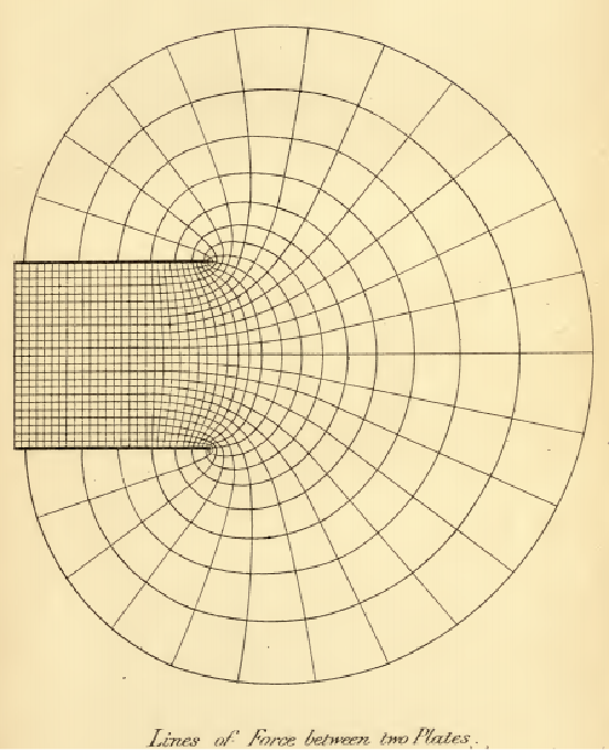

f[z_] := z + E^zInverseFunction[f][z]
top = ComplexContourPlot[ReIm[z - ProductLog[1, E^z]], {z, -3π + π I, 2π + 3 π I}]middle = ComplexContourPlot[ReIm[z - ProductLog[0, E^z]], {z, -3π - π I, 2π + π I}, Contours -> {Range[-10, 2, 0.25], Range[-3, 3, 0.5]}]bottom = ComplexContourPlot[ReIm[z - ProductLog[-1, E^z]], {z, -3π - 3π I, 2π - π I}]Show[top, middle, bottom,
Graphics[{Thick, Red, Line[{{-3π, π}, {-1, π}}],
Line[{{-3π, -π}, {-1, -π}}]}],
PlotRange -> All]Other Applications (2)
f[z_] := z^5 - 2z^4 + 10z^3 - 2z^2 + 2z - 4{min, {steps}} = Reap[FindRoot[f[z], {z, 2 + I}, StepMonitor :> Sow[z]]];sg = ComplexListPlot[steps, PlotRange -> All, Joined -> True, PlotStyle -> White, Mesh -> All];cg = ComplexContourPlot[Abs[f[z]], {z, -I, 2 + I}];Show[cg, sg]ComplexContourPlot[Evaluate@Table[Abs[z^2 - E^I θ] == 1, {θ, 0, 2π, (π/4)}], {z, 1.5}]属性和关系 (9)
ComplexContourPlot 是 ContourPlot 的特殊情形:
{ComplexContourPlot[Re[z^2], {z, -2 - 2I, 2 + 2I}],
ContourPlot[Re[(x + I y)^2], {x, -2, 2}, {y, -2, 2}]}如果有两个或更多函数,ComplexContourPlot 自动隐去着色:
{ComplexContourPlot[ReIm[z^2], {z, -2 - 2I, 2 + 2I}],
	ContourPlot[ReIm[(x + I y)^2], {x, -2, 2}, {y, -2, 2}, ContourShading -> None]}
ComplexRegionPlot 在复平面上绘制区域:
ComplexRegionPlot[Abs[Log[z]] < 1, {z, 3}]ComplexPlot 使用颜色显示函数的自变量和幅值:
ComplexPlot[Log[z], {z, 3}]使用 ComplexPlot3D 用  轴作为幅值:
ComplexPlot3D[Log[z], {z, 3}]用 ComplexArrayPlot 绘制复数数组:
ComplexArrayPlot[Table[x ^ 3 + I y ^ 2, {x, -2, 2, 0.1}, {y, -2, 2, 0.1}]]使用 ReImPlot 和 AbsArgPlot 在实数上绘制复数值:
ReImPlot[Log[x], {x, -3, 3}]AbsArgPlot[Log[x], {x, -3, 3}]使用 ComplexListPlot 显示复数在平面上的位置:
ComplexListPlot[RandomComplex[{-3 - 3I, 3 + 3I}, 100]]ComplexStreamPlot 和 ComplexVectorPlot 将复数视为方向:
ComplexStreamPlot[Log[z], {z, 3}]ComplexVectorPlot[Log[z], {z, 3}]可能存在的问题 (1)
由于 Arg[f] 不能大于  ,ComplexContourPlot 通常不对分支切割进行渲染:
ComplexContourPlot[Arg[Log[Gamma[z]]] == π, {z, -5 - 5I, 5 + 5I}]文本
Wolfram Research (2020),ComplexContourPlot,Wolfram 语言函数,https://reference.wolfram.com/language/ref/ComplexContourPlot.html.
CMS
Wolfram 语言. 2020. "ComplexContourPlot." Wolfram 语言与系统参考资料中心. Wolfram Research. https://reference.wolfram.com/language/ref/ComplexContourPlot.html.
APA
Wolfram 语言. (2020). ComplexContourPlot. Wolfram 语言与系统参考资料中心. 追溯自 https://reference.wolfram.com/language/ref/ComplexContourPlot.html 年