Line


Line
更多信息和选项
- Line 亦称为多段线或线段.
- Line 可被用作几何区域及图形基元.
- Line 表示分段的线段,其中从 pi 到 pi+1 的线段由下式表示
 .
- Line 可用在 Graphics 和 Graphics3D 中.
- 在图形中,点 pi 可以是 Scaled、Offset、ImageScaled 和 Dynamic 表达式.
- 有些指令,比如 Thickness、Dashing、JoinForm、CapForm 和着色会影响图形渲染.
- 在图形中可使用下述选项和设置:
-
VertexColors None 进行插值着色时顶点的颜色 VertexNormals None 显示明暗度用的有效顶点法线 - Line 可以与 GeometricScene 中的符号点一起使用.
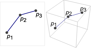
背景
- Line 是一个图形和几何基元,表示一个几何线段或相连的线段序列(折线). 在
 -维空间中,连接
 个点的 Line 的位置由
 个子列表组成的变量列表确定,每个子列表包含
 个直角坐标值. Line 对象的子列表中的坐标值可以是精确的,也可以是近似值,其中,可以用 RegionEmbeddingDimension 来确定所给 Line 表达式的维度
 . 一组线段(或折线)还可以用一个嵌套在单个 Line 基元(“多线段”)中的
 -元组表示. Line 对象的坐标值可以是精确的,也可以是近似值.
- 可以分别使用 Graphics 和 Graphics3D 在二维空间或三维空间显示 Line 对象. 通过使用 GeoGraphics 和 GeoPosition(例如 GeoGraphics[Line[GeoPosition[{{38.9,-77.0},{40.1,-88.3}}]]]),Line 对象还可以用在地图中. 另外,也可用 Line 来定义一个进行某种计算用的区域.
- 尽管线段自身的维度为 1(见 RegionDimension 函数的结果),粗细为零,但在格式化的图形表达式的缺省输出中,Line 对象被显示为看起来有粗细的一条线,而不是一条一维的数学意义上的线段. 而且在图形可视化中,不管从哪个角度看,距离有多远,图形中的线的尺寸不变. 如果想要改变 Line 对象的样式,可以使用调整粗细的指令,比如 Thickness、AbsoluteThickness、Thick 和 Thin;还有改变线的虚实的指令,比如 Dashing、AbsoluteDashing、Dashed、Dotted 和 DotDashed;指定边和线帽形状的指令,有 EdgeForm 和 CapForm;着色指令,比如 Red,规定透明度的指令 Opacity;以及样式选项 Antialiasing. 此外,可以用 VertexColors 指定多条线段的颜色,而 Graphics3D 中的阴影和模拟光照则可使用 VertexNormals 指令来实现.
- 我们可以使用 GeometricTransformation 和更具体的转换函数,比如 Translate 和 Rotate,来改变图形输出中 Line 对象所在的坐标系,而保持产生该输出的 Line 表达式不变.
- 其他图形基元,如 Tube、Arrow、HalfLine 及 InfiniteLine 和样式经过调整的 Line 对象类似. 但是折线仅由直线段组成,如果想要生成光滑的曲线,可以利用 BSplineCurve、BezierCurve 指令产生样条曲线,或者通过插值函数 Interpolation. 有一个和 Line 作为几何区域有关的函数 Interval,它将一对数字作为一个线段在数轴上的端点,并可对它直接进行算术及关系运算.
- 尽管 Line 基元可以出现在图形和定义几何区域的表达式中,但我们要注意到,在 Wolfram 语言里,其他情况下坐标通常都以列表形式表示. 许多图形函数,包括 Plot、ParametricPlot、ParametricPlot3D 和 ContourPlot,返回的图形表达式中会显式包含 Line 对象.
范例
打开所有单元 关闭所有单元基本范例 (4)
Graphics[Line[{{1, 0}, {2, 1}, {3, 0}, {4, 1}}]]Graphics3D[Line[{{1, 1, -1}, {2, 2, 1}, {3, 3, -1}, {4, 4, 1}}]]l = Line[{{1, 0}, {2, 1}, {3, 0}, {4, 1}, {5, 0}, {6, 1}}];{Graphics[{Dashed, l}], Graphics[{Pink, l}], Graphics[{Thick, l}], Graphics[{Thick, Dashed, Pink, l}]}l = Line[{{1, 1, -1}, {2, 2, 1}, {3, 3, -1}, {4, 4, 1}}];{Graphics3D[{Dashed, l}], Graphics3D[{Pink, l}], Graphics3D[{Thick, l}], Graphics3D[{Thick, Dashed, Pink, l}]}计算线段的 ArcLength:
ArcLength[Line[{{0, 0}, {1, 1}}]]RegionCentroid[Line[{{0, 0}, {1, 1}}]]范围 (24)
图形 (14)
规范 (3)
样式 (8)
Table[Graphics[{Thickness[i], Line[{{0, 0}, {2, 1}}]}], {i, {Tiny, Small, Medium, Large}}]Table[Graphics[{t, Line[{{0, 0}, {2, 1}}]}], {t, {Thin, Thick}}]Table[Graphics[{Thickness[i], Line[{{0, 0}, {2, 1}}]}], {i, {.005, .05, .1}}]Table[Graphics[{AbsoluteThickness[i], Line[{{0, 0}, {2, 1}}]}], {i, {1, 5, 10}}]Table[Graphics[{Dashing[i], Line[{{0, 0}, {2, 1}}]}], {i, {Tiny, Small, Medium, Large}}]Table[Graphics[{d, Line[{{0, 0}, {2, 1}}]}], {d, {Dotted, Dashed, DotDashed}}]Table[Graphics[{c, Line[{{0, 0}, {2, 1}}]}], {c, {Red, Green, Blue, Yellow}}]可以用 CapForm 来指定线帽的形状:
Table[Graphics[{CapForm[cap], Thickness[.2], Line[{{-1, -1}, {1, 1}}]}, PlotRange -> 1.5, PlotLabel -> cap], {cap, {"Butt", "Round", "Square"}}]Table[Graphics3D[{CapForm[cap], Thickness[.1], Line[{{-1, -1, -1}, {1, 1, 1}}]}, PlotRange -> 1.5, PlotLabel -> cap], {cap, {"Butt", "Round", "Square"}}]可以用 JoinForm 指定线段连接处的形状:
Table[Graphics[{JoinForm[j], Thickness[.2], Line[{{-1, -0.5}, {0, 0.5}, {1, -0.5}}]}, PlotRange -> 1.5, PlotLabel -> j], {j, {"Bevel", "Round", "Miter"}}]Table[Graphics3D[{JoinForm[j], Thickness[.1], Line[{{-1, -1, -1}, {0, 0, 1}, {1, 1, -1}}]}, PlotRange -> 1.5, PlotLabel -> j], {j, {"Bevel", "Round", "Miter"}}]可以用 VertexColors 指定顶点处的颜色:
Graphics[{Thick, Line[{{0, 0}, {2, 1}}, VertexColors -> {Red, Green}]}]Graphics3D[{Thick, Line[{{0, 0, 0}, {2, 1, 1}}, VertexColors -> {Red, Green}]}]对于三维线段,用 VertexNormals 指定顶点法线:
Graphics3D[{Thick, Yellow, Line[{{0, 0, 0}, {2, 1, 1}}, VertexNormals -> {{1, -1, 1}, {-1, 1, -1}}]}]坐标 (3)
使用 Scaled 的坐标:
Graphics[Line[{Scaled[{0, .2}], Scaled[{1, .8}]}], Frame -> True]Graphics3D[Line[{Scaled[{0, .2, 0}], Scaled[{1, .8, 1}]}], Axes -> True]在二维中使用 ImageScaled 的坐标:
Graphics[Line[{ImageScaled[{0, .2}], ImageScaled[{1, .8}]}], Frame -> True]在二维中使用 Offset 的坐标:
Graphics[Line[{Offset[{10, 20}, {0, 0}], Offset[{-10, -20}, {1, 1}]}], Frame -> True]区域 (10)
RegionEmbeddingDimension[Line[{{1, 2}, {3, 4}}]]RegionEmbeddingDimension[Line[{{1, 2, 3}, {4, 5, 6}}]]RegionDimension[Line[{{1, 2}, {3, 4}}]]RegionDimension[Line[{{1, 2}, {1, 2}}]]ℛ = Line[{{1, 2}, {3, 4}}];{RegionMember[ℛ, {2, 3}], RegionMember[ℛ, {0, 0}]}RegionMember[ℛ, {x, y}]ℛ = Line[{{1, 2}, {3, 4}, {5, 2}}];{RegionMeasure[ℛ], ArcLength[ℛ]}c = RegionCentroid[ℛ]Graphics[{{Gray, ℛ}, {Red, Point[c]}}]ℛ = Line[{{1, 2}, {3, 4}, {5, 2}}];RegionDistance[ℛ, {2, 1}]{Plot3D[RegionDistance[ℛ, {x, y}], {x, -1, 7}, {y, 0, 6}, MeshFunctions -> {#3&}, Mesh -> 5], ContourPlot[RegionDistance[ℛ, {x, y}], {x, -1, 7}, {y, 0, 6}, Contours -> {{0.5, Red}, {1, Green}, {1.5, Blue}}]}ℛ = Line[{{1, 2}, {3, 4}, {5, 2}}];SignedRegionDistance[ℛ, {2, 1}]Plot3D[SignedRegionDistance[ℛ, {x, y}], {x, -1, 7}, {y, 0, 6}, Mesh -> None]ℛ = Line[{{1, 2}, {3, 4}, {1, 6}}];RegionNearest[ℛ, {2, 1}]pts = Table[{2, 4} + 5 / 2{Cos[k 2 π / 25], Sin[k 2π / 25]}, {k, 0., 24}];
nst = RegionNearest[ℛ, #]& /@ pts;Legended[Graphics[{ℛ, {Thin, Gray, Line[Transpose[{pts, nst}]]}, {Red, Point[pts]}, {Blue, Point[nst]}}], PointLegend[{Red, Blue}, {"start", "nearest"}]]ℛ = Line[{{1, 2}, {3, 4}}];BoundedRegionQ[ℛ]rr = RegionBounds[ℛ]Graphics[{ℛ, {EdgeForm[{Dashed, Red}], Opacity[0.2, Yellow], Cuboid@@Transpose[rr]}}]ℛ = Line[{{1, 2}, {3, 4}, {1, 6}}];Integrate[x y, {x, y}∈ℛ]ℛ = Line[{{1, 2}, {3, 4}, {1, 6}}];Minimize[{x y - x, {x, y}∈ℛ}, {x, y}]ℛ = Line[{{0, 0}, {1, 1}, {2, 0}}];Solve[(x - 1)^2 + (y - 1)^2 == 1 && {x, y}∈ℛ, {x, y}]Graphics[{{Thin, ℛ}, {Thin, Circle[{1, 1}]}, {Red, Point[{x, y} /. %]}}, Frame -> True]选项 (3)
VertexColors (2)
应用 (6)
p = Tuples[Table[{Cos[t], Sin[t]}, {t, 0, 2Pi, 2Pi / 11}], 2];Graphics[Line[p]]f[x_] := x ^ 2p = Table[{{a - 2, f'[a]((a - 2) - a) + f[a]}, {a + 2, f'[a]((a + 2) - a) + f[a]}}, {a, -10, 10, .1}];Graphics[Line[p], PlotRange -> {{-1, 1}, {-1, 1}}]Graphics[{Table[Line[{{x, y}, {x, y} + {y, x} / 5 - 1}], {x, 0, 10}, {y, 0, 10}]}, AspectRatio -> 1]Graphics[Line[Accumulate[RandomChoice[{{-1, 0}, {1, 0}, {0, 1}, {0, -1}}, 1000]]]]Graphics3D[Line[Accumulate[RandomChoice[Join[IdentityMatrix[3], -IdentityMatrix[3]], 500]]]]用 Line 代替 Polygon 可以获得特殊的渲染效果:
LineRendering[g_] := g /. Polygon[pt_] :> Line[pt, VertexColors -> Automatic, VertexNormals -> Automatic]Plot3D[Sin[x y], {x, 0, 3}, {y, 0, 3}, Mesh -> False]//LineRenderingPlot3D[Sin[x y ^ 2], {x, 0, 4}, {y, 0, 2}, ColorFunction -> "TemperatureMap", Mesh -> None, Lighting -> Automatic]//LineRenderingobj = RevolutionPlot3D[{8 + Cos[t], 2Sin[t]}, {t, 0, 2Pi}, Mesh -> None, PlotStyle -> FaceForm[None], Axes -> False];Table[Show[obj, Lighting -> ({"Spot", ColorData["SouthwestColors"][RandomReal[]], Scaled[#], {Pi / 4, 100}}&) /@ RandomReal[{-4, 4}, {5, 3}]], {3}]//LineRendering{ExampleData[{"Geometry3D", "Deimos"}], ExampleData[{"Geometry3D", "Vase"}]}//LineRenderingf[x_] := Sin[x ^ 2];lineApprox[f_, n_, xmin_, xmax_] := Module[{vals}, vals = Table[{x, f[x]}, {x, xmin, xmax, (xmax - xmin) / n}];Line@Partition[Riffle[Most@vals, Rest@vals], 2]]lines = lineApprox[f, 30, -4, 4];Show[Plot[f[x], {x, -4, 4}], Graphics[lines]]Integrate[Sqrt[1 + f'[x] ^ 2], {x, -4, 4}]//NArcLength[lines]//NArcLength[lineApprox[f, 300, -4, 4]]//N属性和关系 (4)
可以生成 Line 对象的几个绘图函数:
data = RandomInteger[10, {10}];ListLinePlot[data]ListLinePlot[data, PlotStyle -> DotDashed]% /. Line -> ArrowParametricPlot3D[{Cos[θ], Sin[θ], θ / 4}, {θ, 0, 3Pi}, PlotStyle -> Directive[Thick, Pink]]% /. Line[p_List] :> Point[p]ImplicitRegion 可用来表示任意 Line 区域:
Subscript[ℛ, 1] = Line[{{0, 0}, {1, 1}}];
Subscript[ℛ, 2] = ImplicitRegion[x == y && 0 ≤ x ≤ 1, {x, y}];RegionEqual[Subscript[ℛ, 1], Subscript[ℛ, 2]]ParametricRegion 可用来表示任意 Line 区域:
Subscript[ℛ, 1] = RegionUnion[ParametricRegion[{{1 + t, 2 + t}, 0 ≤ t ≤ 2}, {t}], ParametricRegion[{{3 - t, 4 + t}, 0 ≤ t ≤ 2}, {t}]];
Subscript[ℛ, 2] = Line[{{1, 2}, {3, 4}, {1, 6}}];RegionEqual[Subscript[ℛ, 1], Subscript[ℛ, 2]]可能存在的问题 (1)
必须用机器可以表示的数字来指定 Line 对象:
Graphics[Line[{{0, 0}, {10. ^ 500, 10. ^ 500}}]]MachineNumberQ[10. ^ 500]巧妙范例 (4)
Graphics[Table[{Hue[RandomReal[]], Line[RandomReal[1, {2, 2}]]}, {100}]]Graphics3D[Table[{Hue[RandomReal[]], Line[RandomReal[1, {2, 3}]]}, {100}]]Block[{sp = Normalize /@ RandomReal[{-1, 1}, {500, 3}]},
Graphics3D[{Line[sp, VertexNormals -> sp]}]]Graphics[Table[Line[{{{x, 0}, {1 - x, 1}}, {{0, x}, {1, 1 - x}}}], {x, 0, 1, .02}]]With[{f = {Cos[x] + Sin[x], Sin[x]}}, Graphics[Table[{Hue[t / (2Pi), 1, .8], Line[{f, Normalize[D[f, x]] + f}]} /. x -> t, {t, 0, 2Pi, .1}]]]相关链接

 《Wolfram 语言入门》:坐标与图形
Wolfram Research (1988),Line,Wolfram 语言函数,https://reference.wolfram.com/language/ref/Line.html (更新于 2014 年).
文本
Wolfram Research (1988),Line,Wolfram 语言函数,https://reference.wolfram.com/language/ref/Line.html (更新于 2014 年).
CMS
Wolfram 语言. 1988. "Line." Wolfram 语言与系统参考资料中心. Wolfram Research. 最新版本 2014. https://reference.wolfram.com/language/ref/Line.html.
APA
Wolfram 语言. (1988). Line. Wolfram 语言与系统参考资料中心. 追溯自 https://reference.wolfram.com/language/ref/Line.html 年