


GeoGraphics
GeoGraphics[primitives,options]
represents a two-dimensional geographical image.
Details and Options
- GeoGraphics constructs maps of regions of the world or other celestial bodies.
- GeoGraphics takes a set of geo graphics primitives, does a projection and returns a graphical image.
- GeoGraphics uses the same primitives as Graphics, with the following additions:
-
GeoBoundsRegion[ranges] latitude-longitude rectangle GeoBoundsRegionBoundary[ranges] boundary of a latitude-longitude rectangle GeoCircle[pt,r] cartographic circle supporting geo entities GeoDisk[pt,r] cartographic disk area supporting geo entities GeoHemisphere[pt] hemisphere centered at position pt GeoHemisphereBoundary[pt] boundary of a hemisphere, i.e. a great circle or ellipse GeoMarker[pts] pushpin supporting geo entities GeoPath[pts] cartographic path supporting geo entities GeoPolygon[pts] cartographic polygon supporting geo entities GeoVisibleRegion[pt] visible area from an elevated point GeoVisibleRegionBoundary[pt] horizon from an elevated point DayHemisphere[date] half of Earth illuminated by the Sun at a given time NightHemisphere[date] half of Earth not illuminated by the Sun at a given time DayNightTerminator[date] closed path separating the day and night hemispheres - GeoGraphics uses the same directives as Graphics, with the following addition:
-
GeoStyling[mapstyle] display faces of filled geo objects using mapstyle - GeoGraphics has the same options as Graphics, with the following additions and changes: [List of all options]
-
GeoBackground Automatic style specifications for the background GeoCenter Automatic center coordinates to use GeoGridLines None geographic grid lines to draw GeoGridLinesStyle Automatic style specifications for geographic grid lines GeoGridRange All projected coordinate range to include GeoGridRangePadding Automatic how much to pad the projected range GeoModel Automatic model of the Earth (or other body) to use GeoProjection Automatic projection to use GeoRange Automatic geographic area range to include GeoRangePadding Automatic how much to pad the geographic range GeoResolution Automatic average distance between background pixels GeoScaleBar None scale bar to display GeoServer Automatic specification of a tile server GeoZoomLevel Automatic zoom to use for geographic background MetaInformation {} meta-information about the map RasterSize Automatic raster dimensions for the background data - GeoGraphics can use vector backgrounds like "Terrain", "Plain" or "Classic", and also raster backgrounds like "StreetMap", "Satellite" or "ReliefMap". The default geo background is "Terrain".
- GeoGraphics[] gives a map of the world centered at the longitude of the current geo location with default geo styling.
- AbsoluteOptions can be used to give explicit values for geo graphics settings.
- GeoGraphics is displayed in StandardForm as a graphical image.
- Using GeoGraphics requires internet connectivity.
- Clicking on a geo graphic and selecting the Get Coordinates tool from the Graphics ▶ Drawing Tools allows coordinate information to be interactively read off.
List of all options
Examples
open all close allBasic Examples (7)
Show a map of the world centered at your location:
GeoGraphics[]Display a street map centered on your current location:
GeoGraphics[GeoMarker[], GeoRange -> Quantity[1, "Miles"]]GeoGraphics[Polygon[Entity["Country", "Italy"]]]Style a geo polygon with graphics directives:
GeoGraphics[{EdgeForm[Black], FaceForm[StandardRed], Polygon[Entity["Country", "Italy"]]}]Display a map of France and areas around it:
GeoGraphics[GeoRange -> Entity["Country", "France"], GeoRangePadding -> Quantity[100, "Kilometers"]]GeoGraphics[{GeoStyling["StreetMap"], Polygon[Entity["Country", "Germany"]]}, GeoBackground -> None]Plot the world in a Robinson projection:
GeoGraphics[GeoRange -> "World", GeoProjection -> "Robinson"]Connect two points on Earth with GeoPath:
With[{locations = {GeoPosition[{-35, -55}], GeoPosition[{70, 100}]}}, GeoGraphics[{{StandardRed, GeoPath[locations, "Geodesic"]}}, GeoRange -> "World", GeoProjection -> "Robinson"]]A map of the area around Olympus Mons on Mars:
GeoGraphics[Entity["SolarSystemFeature", "OlympusMonsMars"], GeoRange -> Quantity[400, "Miles"]]Scope (31)
Primitives (20)
GeoGraphics[Polygon[Entity["Country", "UnitedStates"]]]Plot the bounding rectangle of the US, with sides being parallels and meridians:
GeoGraphics[GeoBoundsRegion[Entity["Country", "UnitedStates"]]]Draw a straight line between two cities:
GeoGraphics[{
	Polygon[Entity["Country", "UnitedStates"]],
	StandardRed, Thick, Line[{Entity["City", {"LosAngeles", "California", "UnitedStates"}], Entity["City", {"NewYork", "NewYork", "UnitedStates"}]}]
	}]
Draw a red point at the position of Washington, DC:
GeoGraphics[{StandardRed, PointSize[Large], Point[GeoPosition[Entity["City", {"Washington", "DistrictOfColumbia", "UnitedStates"}]]]}]Draw points at the positions of buildings of the Acropolis:
GeoGraphics[{StandardRed, PointSize[Large], Point[EntityClass["Building", "AcropolisAthens"]]}]Show the location of Madrid with a geo marker:
GeoGraphics[GeoMarker[Entity["City", {"Madrid", "Madrid", "Spain"}]], GeoRange -> Entity["Country", "Spain"]]Plot a set of styled geo disks using different center specifications:
With[{r = Quantity[450, "Kilometers"]},
	GeoGraphics[{
	Yellow, GeoDisk[{40, -4}, r],
	Red, GeoDisk[GeoPosition[{47, 3}], r],
	Blue, GeoDisk[Entity["City", {"Berlin", "Berlin", "Germany"}], r]
	}]]
Plot a set of styled geo circles using different center specifications:
With[{r = Quantity[1000, "Kilometers"]},
	GeoGraphics[{
	Purple, GeoCircle[{40, 0}, r],
	Red, GeoCircle[GeoPosition[Entity["City", {"Nairobi", "Nairobi", "Kenya"}]], r],
	Green, GeoCircle[Entity["City", {"Johannesburg", "Gauteng", "SouthAfrica"}], r]
	}]]
Color the part of the Earth currently in daylight:
GeoGraphics[{Yellow, DayHemisphere[]}, GeoRange -> "World"]Color the part of the Earth currently in darkness:
GeoGraphics[NightHemisphere[], GeoRange -> "World"]Display the current terminator separating daylight from darkness on the Earth:
GeoGraphics[{Red, DayNightTerminator[]}, GeoRange -> "World"]Show the shortest path (geodesic) between New York and Hong Kong:
With[{cities = {Entity["City", {"NewYork", "NewYork", "UnitedStates"}], Entity["City", {"HongKong", "HongKong", "HongKong"}]}},
	GeoGraphics[{GeoPath[cities], Red, Point[cities]}, GeoCenter -> {0, -150}, GeoRange -> "World", Frame -> True]]
Plot a random path of 70 geodesic steps of 1000 kilometers:
GeoGraphics[GeoPath[Flatten@{GeoPosition[{0, 0}], Table[GeoDisplacement[{10 ^ 6, RandomReal[{0, 360}]}], {70}]}, VertexColors -> Table[Hue[i / 100], {i, 0, 70}]]]Draw an arrow between two cities:
GeoGraphics[{Polygon[Entity["Country", "UnitedStates"]], Red, Arrow[{Entity["City", {"LosAngeles", "California", "UnitedStates"}], Entity["City", {"NewYork", "NewYork", "UnitedStates"}]}]}]Draw an arrow with multiple segments:
GeoGraphics[{Polygon[Entity["Country", "UnitedStates"]], Red, Arrow[{Entity["City", {"LosAngeles", "California", "UnitedStates"}], Entity["City", {"NewYork", "NewYork", "UnitedStates"}], Entity["City", {"Miami", "Florida", "UnitedStates"}]}]}]The visible region from an altitude of 10 km:
GeoGraphics[GeoVisibleRegion[{40, -90, 10000}]]The boundary of the visible region from an altitude of 10 km:
GeoGraphics[GeoVisibleRegionBoundary[{40, -90, 10000}]]Smooth country polygons using geo filled curves:
polygonToFilledCurve[Polygon[GeoPosition[l_]]] := FilledCurve[BSplineCurve[GeoPosition[#], SplineDegree -> Round[Length[#] / 4]]]& /@ lShow a map of smoothed South American nations:
GeoGraphics[{GeoStyling[Opacity[0.6]], RandomColor[], polygonToFilledCurve[#]}& /@ CountryData[EntityClass["Country", "SouthAmerica"], "SchematicPolygon"]]Plot the area around the Arctic Circle:
GeoGraphics[{Point[GeoPosition[{90, 0}]], Text[Column[{"North", "Pole"}], GeoPosition[{90, -80}]], Orange, Thick, Text[Style["Arctic Circle", Bold, Medium], GeoPosition[{65, 225}], Automatic, {1, 1}], Dashed, GeoPath["ArcticCircle"]}, GeoProjection -> {"LambertAzimuthal", "Centering" -> {90, 0}}, GeoRange -> {{60, 90}, All}, GeoRangePadding -> Full]Combine a number of geo graphics primitives in one map:
GeoGraphics[{
	Polygon[Entity["Country", "Austria"]], {GeoStyling["ReliefMap"], Polygon[Entity["Country", "Hungary"]]},
	Red, Polygon[Entity["Country", "Switzerland"]], PointSize[Large], Tooltip[Point[Entity["City", {"Budapest", "Budapest", "Hungary"}]], [image]],   {GeoStyling[{"GeoImage", [image]}], Polygon[Entity["Country", "Slovenia"]]}, {GeoStyling["ContourMap", ColorFunction -> ColorData["GreenPinkTones"]], GeoDisk[Entity["City", {"Krakow", "Malopolskie", "Poland"}], Quantity[120, "Kilometers"]]}, Directive[{Purple, Thickness[Small]}], Arrow[GeoPath[{Entity["City", {"Stuttgart", "BadenWurttemberg", "Germany"}], Entity["City", {"Zurich", "Zurich", "Switzerland"}]}]]
	}, GeoCenter -> Entity["City", {"Vienna", "Vienna", "Austria"}], GeoGridLines -> Automatic, GeoGridLinesStyle -> Directive[{Opacity[0.7], Orange}],
	GeoZoomLevel -> 6, ImageSize -> Large]
GeoGraphics supports 2D and 3D graphics primitives:
GeoGraphics[{
	Simplex[GeoPosition[{{0, 0}, {-40, 0}, {-30, 80}}]], Ball[GeoPosition[{-10, -30}], 0.2], Ellipsoid[GeoPosition[{50, -100}], {0.2, 0.4}], Parallelepiped[GeoPosition[{0, -160}], {{0.2, 0}, {0.3, 0.4}}], Parallelogram[GeoPosition[{-40, -130}], {{0.2, 0}, {0.3, -0.5}}], Sphere[GeoPosition[{70, 120}], 0.4]
	},
	GeoProjection -> "Bonne", GeoRange -> "World"
	]
Projections and Map Coordinates (8)
Large-scale maps use the equirectangular projection by default:
GeoGraphics[GeoRange -> "World"]AbsoluteOptions[%, GeoProjection]Intermediate-scale maps use the Lambert azimuthal projection centered at the geo range of the map:
GeoGraphics[Entity["Country", "UnitedStates"]]AbsoluteOptions[%, GeoProjection]Small scales are represented by default using the Mercator projection, to preserve angles:
GeoGraphics[Entity["City", {"Paris", "IleDeFrance", "France"}], GeoRange -> Quantity[10, "Kilometers"]]AbsoluteOptions[%, GeoProjection]Choose a projection with default parameters from GeoProjectionData[]:
GeoGraphics[Polygon[Entity["Country", "Tunisia"]], GeoProjection -> "WinkelTripel"]GeoGraphics[Polygon[EntityClass["Country", "Europe"]], GeoProjection -> "Orthographic"]Specify the parameters of a cylindrical projection using the default center meridian at Greenwich:
GeoGraphics[GeoRange -> "World", GeoProjection -> "Mercator", Frame -> True]For cylindrical projections, easting represents longitude and is returned in degrees. Use radians instead:
GeoGraphics[GeoRange -> "World", GeoProjection -> {"Mercator", "ReferenceModel" -> 1},
	Frame -> True]
Use a scale in kilometers for equatorial distance. The same radius geo disks show distance distortion:
GeoGraphics[Table[GeoDisk[{lat, lon}, Quantity[1000, "Kilometers"]], {lat, -60, 60, 20}, {lon, -140, 140, 40}], GeoRange -> "World", GeoProjection -> {"Mercator", "ReferenceModel" -> 6378.137},
	Frame -> True]
Specify the parameters of an azimuthal projection, mainly the tangency point of the projection plane:
GeoGraphics[Polygon[Entity["Country", "Brazil"]], GeoProjection -> {"Orthographic", "Centering" -> Entity["City", {"RioDeJaneiro", "RioDeJaneiro", "Brazil"}]}]GeoGraphics[Polygon[Entity["Country", "Brazil"]], GeoProjection -> {"Orthographic", "Centering" -> Entity["City", {"NewYork", "NewYork", "UnitedStates"}]}, Background -> Black]Some azimuthal projections cannot cover the whole world in a single map; the Lambert azimuthal projection can:
GeoGraphics[GeoRange -> "World", GeoProjection -> "LambertAzimuthal"]Specify the parameters of a conic projection by choosing a centering point:
GeoGraphics[GeoRange -> "World", GeoProjection -> {"ConicEquidistant", "Centering" -> {0, 0}}, Axes -> True]Choose the standard parallels, which are true to scale, and draw them:
GeoGraphics[{GeoPath[{"Parallel", 60}], GeoPath[{"Parallel", 70}]}, GeoRange -> "World", GeoProjection -> {"ConicEquidistant", "StandardParallels" -> {60, 70}}]GeoGraphics[{GeoPath[{"Parallel", -40}], GeoPath[{"Parallel", 70}]}, GeoRange -> "World", GeoProjection -> {"ConicEquidistant", "StandardParallels" -> {-40, 70}}]Geo primitives are defined in terms of {lat,lon} positions on the Earth and they are projected:
GeoGraphics[{Purple, GeoDisk[{-30, 70}, Quantity[5000, "Kilometers"]]}, GeoRange -> "World", GeoProjection -> "Bonne", Frame -> True]Standard primitives are defined in terms of map coordinates and they are not projected:
GeoGraphics[{
	Purple, GeoDisk[{-30, 70}, Quantity[5000, "Kilometers"]],
	Orange, Disk[{-1, .5}, .5]
	}, GeoRange -> "World", GeoProjection -> "Bonne", Frame -> True]
Standard primitives may be placed using GeoPosition[{lat,lon}], which is automatically projected:
GeoGraphics[{
	Purple, GeoDisk[{-30, 70}, Quantity[5000, "Kilometers"]],
	Orange, Disk[GeoPosition[{-30, 70}], .5]
	}, GeoRange -> "World", GeoProjection -> "Bonne", Frame -> True]
A GeoPath (geodesic or loxodrome) is generically curved in the map:
GeoGraphics[GeoPath[{{-30, -120}, {80, 10}}], GeoProjection -> "Equirectangular", Frame -> True]The standard Line primitive is always a straight line in the map:
GeoGraphics[{GeoPath[{{-30, -120}, {80, 10}}], Red, Line[{{-120, -30}, {10, 80}}]}, GeoProjection -> "Equirectangular", Frame -> True]Coordinates coincide (though reversed) only for the equirectangular projection; use GeoPosition otherwise:
GeoGraphics[{GeoPath[{{-30, -120}, {80, 10}}], Red, Line[GeoPosition[{{-30, -120}, {80, 10}}]]}, GeoProjection -> "Cassini", Frame -> True]A filled GeoPath has generically curved sides in the map:
points = {{-40, -50}, {40, -30}, {40, 30}, {-40, 50}, {-40, -50}};GeoGraphics[{Purple, FilledCurve[GeoPath[points]]}, GeoProjection -> "Albers"]The standard Polygon primitive always has straight sides:
GeoGraphics[{Orange, Polygon[GeoPosition[points]]}, GeoProjection -> "Albers"]GeoGraphics[{
Purple, FilledCurve[GeoPath[points]],
Orange, Polygon[GeoPosition[points]]
}, GeoProjection -> "Albers"]Coordinates (3)
Coordinate ranges for the map are determined by the total bounding box of all coordinates:
GeoGraphics[{Orange, Polygon[EntityClass["Country", "Europe"]]}]Coordinate specifications outside primitives contribute to the bounding box, but are not plotted:
GeoGraphics[{GeoPosition[{50, 20}], Entity["Country", "Portugal"]}]Therefore this produces a map around a given geographical entity, with default geo range padding:
GeoGraphics[Entity["Country", "France"]]Coordinates in Graphics primitives that are not wrapped in GeoPosition are considered to be already in final projection. They also count toward the total coordinates range:
GeoGraphics[{GeoStyling["OutlineMap"], Opacity[.5], EdgeForm[Thin], Polygon[Entity["Country", "Germany"]], Polygon[{{0, 55}, {20, 55}, {20, 65}, {0, 65}}]}, GeoProjection -> "Mercator", Frame -> True]Options (22)
GeoBackground (5)
Use the default background for map region and background:
GeoGraphics[{Polygon[Entity["Country", "UnitedStates"]]}]Draw a relief map background for a map of the US:
GeoGraphics[{Polygon[Entity["Country", "UnitedStates"]]}, GeoBackground -> GeoStyling["ReliefMap"]]Use a relief map background for world maps with various projections:
GeoGraphics[GeoProjection -> #, GeoGridLines -> Automatic, GeoRange -> All, GeoBackground -> GeoStyling["ReliefMap"], GeoGridLinesStyle -> Directive[Opacity[.5], Yellow]]& /@ {"LambertAzimuthal", "Mercator", "Equirectangular", "Bonne"}Specify a uniform background for the geographic map:
GeoGraphics[Polygon[Entity["Country", "World"]], GeoGridLines -> Automatic, GeoRange -> All, GeoBackground -> GeoStyling[LightBlue], GeoProjection -> "Bonne"]Specify uniform backgrounds for the map and graphic as a whole:
GeoGraphics[Polygon[Entity["Country", "World"]], GeoGridLines -> Automatic, GeoRange -> All, GeoBackground -> GeoStyling[LightBlue], Background -> Blue, GeoProjection -> "Bonne"]World map with country boundaries:
GeoGraphics["World", GeoBackground -> "CountryBorders"]European country borders in 1900:
GeoGraphics[Entity["GeographicRegion", "Europe"], GeoBackground -> Dated["CountryBorders", 1900]]GeoGraphics[Entity["Building", "EiffelTower::5h9w8"], GeoRange -> Quantity[1, "Kilometers"], GeoBackground -> "StreetMap"]GeoGraphics[Entity["AdministrativeDivision", {"Hawaii", "UnitedStates"}], GeoBackground -> "ReliefMap"]GeoGraphics[Entity["Building", "EiffelTower::5h9w8"], GeoRange -> Quantity[1, "Kilometers"], GeoBackground -> "Plain"]GeoGraphics[Entity["AdministrativeDivision", {"Hawaii", "UnitedStates"}], GeoBackground -> "ClassicDark"]GeoCenter (1)
Use GeoCenter to define the center for the map:
GeoGraphics[GeoRange -> "World", GeoCenter -> {0, -180}]The geo range is extended to have Munich at the center of the map:
GeoGraphics[{Polygon[Entity["Country", "Germany"]], GeoMarker[Entity["City", {"Munich", "Bavaria", "Germany"}]]}, GeoCenter -> Entity["City", {"Munich", "Bavaria", "Germany"}]]GeoGridLines (1)
Use GeoGridLines to overlay the map with lines of latitude and longitude:
GeoGraphics[{GeoStyling["ReliefMap"], Polygon[Entity["Country", "UnitedStates"]]}, GeoGridLines -> Automatic]Show geo grid lines (constant latitude and longitude) and grid lines (constant projected coordinates):
GeoGraphics[GeoRange -> "World", GeoBackground -> None, GeoProjection -> "Bonne", GeoGridLines -> Automatic, GridLines -> Automatic]GeoGridLinesStyle (1)
Use GeoGridLinesStyle to change the styling for lines of latitude and longitude:
GeoGraphics[{GeoStyling["ReliefMap"], Polygon[Entity["Country", "UnitedStates"]]}, GeoGridLines -> Automatic, GeoGridLinesStyle -> Yellow, GeoBackground -> Black]GeoGridRange (2)
Specify projected coordinate ranges in the coordinate system determined by the projection:
GeoGraphics[GeoProjection -> "Mercator", GeoGridRange -> {{-120, -60}, {0, 60}}]A map of the Chicago area in zone 16 of the Universal Transverse Mercator coordinate system:
GeoGridPosition[Entity["City", {"Chicago", "Illinois", "UnitedStates"}], "UTMZone16"]GeoGraphics[GeoProjection -> "UTMZone16", GeoBackground -> "Satellite", GeoGridRange -> {{430000, 470000}, {4615000, 4655000}}]GeoGridRangePadding (1)
Add padding in the projected coordinate system:
GeoGraphics["World", GeoProjection -> "Bonne", GeoGridRangePadding -> 0.3]Add positive padding in the horizontal direction, but negative padding in the vertical direction:
GeoGraphics["World", GeoProjection -> "Bonne", GeoGridRangePadding -> {0.5, -0.5}]GeoModel (2)
Construct a geodesic path that leaves Rome with NE direction and goes around the Earth three times:
city = Entity["City", {"Rome", "Lazio", "Italy"}];
r = Quantity[6.367 10^6, "Meters"];
course = GeoDisplacement[{6Pi r, 45}, "Geodesic"]
Computations are performed by default on an ellipsoidal Earth, meaning geodesic paths do not close:
GeoGraphics[Arrow@GeoPath[{city, course}], GeoCenter -> city, GeoRange -> Quantity[150, "Kilometers"]]Using a spherical model for the Earth results in closed geodesics:
GeoGraphics[Arrow@GeoPath[{city, course}], GeoCenter -> city, GeoRange -> Quantity[150, "Kilometers"], GeoModel -> r]GeoGraphics[GeoRange -> All, GeoModel -> "Mars", GeoProjection -> "Mollweide", Background -> Black]GeoProjection (1)
Use GeoProjection to choose the map projection:
GeoGraphics[GeoRange -> "World", GeoProjection -> {"Bonne", "Centering" -> {0, 0}}]GeoRange (1)
Use GeoRange to define the latitude and longitude coordinate ranges:
GeoGraphics[GeoRange -> {{-40, 40}, All}]GeoGraphics[GeoRange -> {All, {-90, 90}}]GeoGraphics[GeoRange -> {{-90, 90}, {-360, 0}}]GeoRangePadding (1)
Use GeoRangePadding to pad the coordinate range for the map:
GeoGraphics[{Polygon[Entity["Country", "UnitedStates"]]}, GeoBackground -> GeoStyling["ReliefMap"], GeoRangePadding -> Scaled[0.2]]GeoResolution (1)
Specify the geo zoom level as an average distance between neighboring pixels:
GeoGraphics[Entity["Building", "EiffelTower::5h9w8"], GeoResolution -> Quantity[100, "Meters"], GeoBackground -> "StreetMap"]GeoGraphics[Entity["Building", "EiffelTower::5h9w8"], GeoResolution -> Quantity[1, "Yards"], GeoBackground -> "StreetMap"]GeoScaleBar (1)
GeoGraphics[Entity["City", {"Champaign", "Illinois", "UnitedStates"}], GeoScaleBar -> None]Display the geo scale in kilometers:
GeoGraphics[Entity["City", {"Champaign", "Illinois", "UnitedStates"}], GeoScaleBar -> "Kilometers"]Show a geo scale in metric and imperial:
GeoGraphics[Entity["City", {"Champaign", "Illinois", "UnitedStates"}], GeoScaleBar -> {"Metric", "Imperial"}]GeoServer (1)
By default, GeoGraphics downloads geo background tiles from the Wolfram geo server:
GeoGraphics[Entity["Country", "UnitedStates"], GeoServer -> Automatic]Use an alternative tile server:
GeoGraphics[Entity["Country", "UnitedStates"], GeoServer -> "http://a.tile.openstreetmap.org/`1`/`2`/`3`.png"]GeoZoomLevel (2)
Display Canada at the default GeoZoomLevel:
GeoGraphics[Entity["Country", "Canada"], GeoBackground -> "Plain"]AbsoluteOptions[%, GeoZoomLevel]Explicitly specify GeoZoomLevel to obtain a more detailed map rendering:
GeoGraphics[Entity["Country", "Canada"], GeoZoomLevel -> 4, GeoBackground -> "Plain"]Display the area around Notre Dame de Paris at different levels of magnification:
(GeoGraphics[{Red, PointSize[Large], Point[Entity["Building", "NotreDameCathedral::95fcw"]]}, GeoRange -> Quantity[100, "Meters"], GeoZoomLevel -> #1]&) /@ Range[11, 16]MetaInformation (1)
Meta-information about the map sources:
GeoGraphics[Polygon[Entity["Country", "Portugal"]]]AbsoluteOptions[%, MetaInformation]Add your own meta-information:
GeoGraphics[Polygon[Entity["Country", "Portugal"]], MetaInformation -> {"Date" -> DateObject[], "GeoLocation" -> $GeoLocation, "UnitSystem" -> $UnitSystem, "CloudEvaluation" -> $CloudEvaluation}]AbsoluteOptions[%, MetaInformation]Applications (9)
Make a map of the 50 states in the US with Alaska and Hawaii as insets:
Hawaii = GeoGraphics[{GeoStyling["OutlineMap"], Polygon[Entity["AdministrativeDivision", {"Hawaii", "UnitedStates"}]]}, GeoBackground -> None]Alaska = GeoGraphics[{GeoStyling["OutlineMap"], Polygon[Entity["AdministrativeDivision", {"Alaska", "UnitedStates"}]]}, GeoBackground -> None]GeoGraphics[{GeoStyling["OutlineMap"], Polygon[Entity["Country", "UnitedStates"]], Inset[Alaska, {-0.21, -0.1}, {0, 0}, 0.3], Inset[Hawaii, {0.02, -0.83}, {-158, -21}, 0.1]}, GeoBackground -> None, GeoProjection -> {"LambertAzimuthal", "Centering" -> GeoPosition[{30, -195 / 2}]}, Frame -> True, FrameTicks -> None, PlotRange -> {{-0.37, 0.38}, {-0.2, 0.38}}]Use polygons, geo circle, and other graphics primitives to build up a geographic map:
GeoGraphics[{
	GeoStyling["ReliefMap"], Polygon[Entity["Country", "Greece"]],
	Dashed, GeoCircle[Entity["City", {"Athens", "Attiki", "Greece"}], Quantity[200, "Kilometers"]],
	Dotted, Line[{Entity["City", {"Athens", "Attiki", "Greece"}], Entity["Island", "Rhodes"]}],
	Red, PointSize[Large], Point[EntityClass["Building", "AcropolisAthens"]]}, GeoBackground -> "StreetMapNoLabels"]
Draw thick arrows between pairs of countries:
thickarrow[l_, t_, m_, {w_, δ_}] := Module[{f, M = 200, l1 = l /. e_Entity :> EntityValue[e, "Coordinates"] /. GeoPosition[s_] :> s}, f = BSplineFunction[Append[Flatten[Table[#1 + k / m (#2 - #1), {k, 0, m - 1}]&@@@Partition[l1, 2, 1], 1], Last[l1]]];
{GeoStyling[Opacity[.8]], Polygon[GeoPosition[Join@@(#1[Table[f[s] + #2 If[s < 1 - δ, 1, w (1 - s) / δ] t Normalize[Reverse[f'[s]] {-1, 1}], {s, 0, 1, 1 / M}]]&@@@{{#&, 1}, {Reverse, -1}})]]}]GeoGraphics[{
GeoStyling[Opacity[.5]], EdgeForm[Black],
Orange, Polygon /@ {Entity["Country", "UnitedStates"], Entity["Country", "SouthAfrica"]},
thickarrow[{Entity["City", {"Chicago", "Illinois", "UnitedStates"}], Entity["City", {"London", "GreaterLondon", "UnitedKingdom"}], Entity["City", {"Moscow", "Moscow", "Russia"}], Entity["City", {"Johannesburg", "Gauteng", "SouthAfrica"}]}, 3, 2, {4, 0.03}],
Blue, Polygon /@ {Entity["Country", "Chile"], Entity["Country", "India"]},
thickarrow[{Entity["City", {"Santiago", "Metropolitana", "Chile"}], Entity["City", {"MexicoCity", "DistritoFederal", "Mexico"}], Entity["City", {"Oslo", "Oslo", "Norway"}], Entity["City", {"Dubai", "Dubai", "UnitedArabEmirates"}], Entity["City", {"NewDelhi", "Delhi", "India"}]}, 6, 2, {4, 0.05}],
Darker[Green], Polygon /@ {Entity["Country", "Australia"], Entity["Country", "Spain"]}, thickarrow[{Entity["City", {"Sydney", "NewSouthWales", "Australia"}], Entity["City", {"Tokyo", "Tokyo", "Japan"}], Entity["City", {"Moscow", "Moscow", "Russia"}], Entity["City", {"Madrid", "Madrid", "Spain"}]}, 4, 2, {3, 0.05}]
}, GeoRange -> All, GeoBackground -> "Monochrome"]Show the configuration of continents on Earth 200 million years ago:
GeoGraphics[{GeoStyling["OutlineMap"], EdgeForm[Gray], GeologicalPeriodData["JurassicPeriod", "ContinentalPlates"][DateObject[{-200000000}]]}, GeoBackground -> LightBlue, GeoRange -> "World", GeoProjection -> "AmericanPolyconic"]Retrieve the epicenter locations of earthquakes in California:
dat = EarthquakeData[Entity["AdministrativeDivision", {"California", "UnitedStates"}], 4, {{1980, 1, 1}, {2014, 12, 31}}, "Position"]["Values"];Plot the epicenters on a map of California:
GeoGraphics[{Polygon[Entity["AdministrativeDivision", {"California", "UnitedStates"}]], StandardRed, PointSize[.02], Point[dat]}]Get the geographic bounds of California:
{{latmin, latmax}, {lonmin, lonmax}} = GeoBounds[Entity["AdministrativeDivision", {"California", "UnitedStates"}]];Make a smooth kernel distribution of the earthquake epicenters:
𝒟 = SmoothKernelDistribution[dat[[All, 1]], "Silverman"];dens = ContourPlot[Evaluate[PDF[𝒟, {y, x}] ^ (1 / 5)], {x, lonmin, lonmax}, {y, latmin, latmax}, Frame -> False, PlotRange -> {0.05, All}, Contours -> 15, ColorFunction -> (Directive[ColorData["TemperatureMap"][#], Opacity[0.5]]&), PlotRangePadding -> None]Show the results on a map with the epicenters themselves shown as black dots:
With[{p = Polygon[Entity["AdministrativeDivision", {"California", "UnitedStates"}]]}, GeoGraphics[{p, GeoStyling[{"GeoImage", dens}], p, Black, Opacity[0.2], PointSize[0.01], Point[dat]}]]Construct street maps of Monaco and Gibraltar:
{monaco, gibraltar} = GeoGraphics[{GeoStyling["StreetMap"], Polygon[#1], GeoStyling["OutlineMap", Directive[Opacity[0.3], #2, EdgeForm[Black]]], Polygon[#1]}, GeoProjection -> "Equirectangular", Frame -> True, GeoBackground -> None]&@@@{{Entity["Country", "Monaco"], Purple}, {Entity["Country", "Gibraltar"], Darker[Green]}}Transplant Monaco (centered at the Trump Building) and Gibraltar (centered at the Brooklyn Central Library) to New York by modifying the coordinates of the polygon:
{monacoinnewyork, gibraltarinnewyork} = With[{mpNY = EntityValue[#3, "Position"][[1]], mp = CountryData[#1, "CenterCoordinates"]},
	#2[[1, 1]] /. Polygon[l_, rest___] :> Polygon[GeoPosition[Map[(Reverse[#] - mp + mpNY)&, l, {-2}]], rest]] &@@@{ {Entity["Country", "Monaco"], monaco, Entity["Building", "TrumpBuilding"]}, {Entity["Country", "Gibraltar"], gibraltar, Entity["Building", "BrooklynPublicLibraryCentralBranch"]}};
Show the shifted Monaco and Gibraltar on top of the city limits of New York:
GeoGraphics[{
	GeoStyling["OutlineMap", Directive[Opacity[0.2], Yellow, EdgeForm[Black]]], Polygon[Entity["City", {"NewYork", "NewYork", "UnitedStates"}]],
	GeoStyling[], monacoinnewyork, gibraltarinnewyork}, GeoProjection -> "Equirectangular", Frame -> True]
Define "Australian" transformation and geo disk centered on Australia:
upsidedown = (ImageTransformation[#, RotationTransform[Pi], DataRange -> {Automatic, {-.5, .5}}]&);downunder = GeoDisk[Entity["Country", "Australia"], Quantity[2000, "Miles"]];Plot Australia from the rest of the world's perspective:
GeoGraphics[{GeoStyling["ReliefMap", GeoStylingImageFunction -> upsidedown], downunder}, GeoBackground -> "StreetMapNoLabels", GeoRange -> "World"][[1]]Plot the rest of the world from Australia's perspective:
Rotate[%, Pi]Compare a historical map of Paris with a modern street map:
paris1775orig = Import["http://upload.wikimedia.org/wikipedia/commons/thumb/4/4a/1775_Plan_de_Jaillot.jpg/893px-1775_Plan_de_Jaillot.jpg"]Crop the elegant yet extraneous frame:
paris1775 = ImageTake[paris1775orig, {80, -60}, {50, -50}]Pick three characteristic points on the two maps and identify them with approximate positions:
places = {placedeconcorde = {GeoPosition[{48.8658, 2.32075}], {0.1623, 0.4396}}, notredame = {GeoPosition[{48.8527, 2.35047}], {0.5087, 0.4910}}, museedehistorie = {GeoPosition[{48.8586, 2.31283}], {0.1691, 0.2702}}};Plot the resulting points on the maps:
With[{colors = {Red, Blue, Darker[Green]}},
	{Graphics[{Raster[Reverse[ImageData[paris1775]], {{0, 0}, {1, 1}}], PointSize[Large], Transpose[{colors, (Point[Last[#1]]&) /@ places}]}], GeoGraphics[{PointSize[Large], Transpose[{colors, (Point[First[#1]]&) /@ places}]},
	GeoRangePadding -> Quantity[3, "Kilometers"], GeoZoomLevel -> 14, GeoBackground -> "StreetMap"]}]
Get a street map of Paris from today:
paristoday = GeoGraphics[{}, GeoCenter -> GeoPosition[{48.8568, 2.3427}], GeoRange -> Quantity[3, "Kilometers"], GeoZoomLevel -> 15, GeoBackground -> "StreetMapNoLabels"]Find an affine transformation that maps the three points from each map into each other:
mercxy[gp_GeoPosition] := GeoGridPosition[gp, GeoProjection /. Options[paristoday]][[1]]transform = AffineTransform[{{{ax, ay}, {bx, by}}, {a, b}}] /.
Solve[Flatten[{{{ax, ay}.#2 + a, {bx, by}.#2 + b} == mercxy[#1]}&@@@places], {a, ax, ay, b, bx, by}][[1]]Color the modern street map in gray and the historical map in red:
With[{ι = ImageApply},
	{parisnew = Graphics[{Raster[Reverse[ImageData[ι[# ^ 2&, ColorConvert[
	Rasterize[paristoday, "Image"], "Grayscale"]]]],
	mercxy[GeoPosition[#]]& /@ Transpose[GeoRange /. Options[paristoday, GeoRange]]]}],
	parisold = ColorCombine[{ι[0.7#&, #], ι[0.&, #], ι[0.&, #], ι[# ^ 2&, #]}, "RGB"]&[ColorConvert[paris1775, "Grayscale"]]}]
Use the preceding affine transformation to show the two aligned maps over each other:
Show[{parisnew, Graphics[GeometricTransformation[
	Raster[Reverse[ImageData[parisold]], {{0, 0}, {1, 1}}], transform]]}]
Smooth out and scale a country by computing a discrete Fourier transform of its boundary:
points = (Append[#1, #1[[1]]]&)[(#1.{1, I}&) /@ Last[SortBy[CountryData["UnitedStates", "Polygon"][[1, 1]], Length]]];fourier[points_, λ_] := Module[{order = Ceiling[Length[points] λ]^2, mp = ({Re[#1], Im[#1]}&)[Mean[points]], μ = Length[points], ft}, ft = (Append[#1, First[#1]]&)[({Re[#1], Im[#1]}&) /@ FourierDCT[FourierDCT[points, 2] Table[If[j ≤ order, 1, 0], {j, μ}], 3]];MapIndexed[mp + λ (#1 - mp)&, ft]]Superimpose scaled geo B-spline versions of the US border on a map:
GeoGraphics[{Polygon[Entity["Country", "UnitedStates"]], LightBlue, BSplineCurve[Table[GeoPosition[fourier[points, λ]], {λ, 0.05, 1, 0.05}]]}]Properties & Relations (7)
GeoGraphics returns a GeoGraphics expression, with a Graphics object in its first argument:
GeoGraphics[Entity["Country", "HongKong"], GeoBackground -> "StreetMap"]{Head[%], Head[First[%]]}GeoImage returns an Image expression, the background image of the previous result:
GeoImage[Entity["Country", "HongKong"], "StreetMap"]Head[%]GeoGraphics behaves like Graphics with standard primitives, but adds a geo background:
Graphics[{Line[{{0, 0}, {120, 30}, {-120, 60}}], Red, Circle[{-60, 30}, 30]}, Frame -> True]Coordinates are interpreted as {lon,lat} angles in the equirectangular projection:
GeoGraphics[{Line[{{0, 0}, {120, 30}, {-120, 60}}], Red, Circle[{-60, 30}, 30]}, Frame -> True]AbsoluteOptions[%, GeoProjection]Add GeoPosition wrappers to use {lat,lon} angles:
GeoGraphics[{Line[GeoPosition[{{0, 0}, {30, 120}, {60, -120}}]], Red, Circle[GeoPosition[{30, -60}], 30]}, Frame -> True]Coordinates inside geo primitives are always given in {lat,lon} angles:
GeoGraphics[{GeoPath[{{0, 0}, {30, 120}, {60, -120}}], Red, GeoCircle[{30, -60}, 3000000]}, Frame -> True]Adding GeoPosition does not modify the result:
GeoGraphics[{GeoPath[GeoPosition[{{0, 0}, {30, 120}, {60, -120}}]], Red, GeoCircle[GeoPosition[{30, -60}], 3000000]}, Frame -> True]GeoRange determines the part of the Earth to plot, before projection:
box = GeoBoundsRegionBoundary[{{0, 60}, {0, 60}}];GeoGraphics[box, GeoRange -> {{0, 60}, {0, 60}}, Frame -> True]projection = Options[%, GeoProjection]PlotRange determines the part of the map to plot, after projection:
GeoGraphics[box, projection, GeoRange -> {{0, 60}, {0, 60}}, Frame -> True, PlotRange -> {{-0.4, 0.4}, {-0.4, 0.4}}]Use GeoRangePadding to extend the geo range:
GeoGraphics[box, GeoRange -> {{0, 60}, {0, 60}}, GeoRangePadding -> Quantity[400, "Miles"], Frame -> True]Use PlotRangePadding to extend the plot range:
GeoGraphics[box, GeoRange -> {{0, 60}, {0, 60}}, PlotRangePadding -> 0.4, Frame -> True]Use GeoRangePaddingFull to automatically extend the geo range to cover the initial plot range:
GeoGraphics[box, GeoRange -> {{0, 60}, {0, 60}}, GeoRangePadding -> Full, Frame -> True]Geographic Entity objects represent the corresponding region or position, but are not geo primitives:
GeoGraphics[{Entity["Country", "Spain"], Entity["City", {"Madrid", "Madrid", "Spain"}]}, GeoBackground -> None, Frame -> True]Use Polygon or Point to draw the respective region or point, with default geo styling:
GeoGraphics[{Polygon[Entity["Country", "Spain"]], Point[Entity["City", {"Madrid", "Madrid", "Spain"}]]}, GeoBackground -> None, Frame -> True]Modify the default geo styling:
GeoGraphics[{GeoStyling["ReliefMap"], Polygon[Entity["Country", "Spain"]], Red, PointSize[Large], Point[Entity["City", {"Madrid", "Madrid", "Spain"}]]}, GeoBackground -> None, Frame -> True]The shapes of entities generically undergo distortion upon projection. Here are default (in this case "Mercator") and "Equirectangular" projections for Sweden:
country = Entity["Country", "Sweden"];maps = {
GeoGraphics[{Yellow, Opacity[0.5], EdgeForm[Thin], Polygon[country]}, Frame -> True], GeoGraphics[{Yellow, Opacity[0.5], EdgeForm[Thin], Polygon[country]}, Frame -> True, GeoProjection -> "Equirectangular"]
}projs = AbsoluteOptions[#, GeoProjection]& /@ mapsUsing GeoGridPosition and an explicit projection, you can project the country by hand:
projectedpolygon = EntityValue[country, "Polygon"] /. gp_GeoPosition :> GeoGridPosition[gp, projs[[1, 1, 2]]][[1]];The coordinates of the manually transformed polygon match the ones from the default projection:
GraphicsRow[{
	maps[[1, 1]],
	Graphics[{Opacity[0.3], Red, EdgeForm[Thin], projectedpolygon}, Frame -> True, Sequence@@AbsoluteOptions[maps[[1]], PlotRange]]
	}, ImageSize -> Small]
Using Line (or Arrow) inside a geo graphic gives a straight line whose points depend on the projection:
GeoGraphics[{
	Polygon[Entity["Country", "UnitedStates"]],
	Red, Thick, Line[{Entity["City", {"LosAngeles", "California", "UnitedStates"}], Entity["City", {"NewYork", "NewYork", "UnitedStates"}]}]}, GeoProjection -> #1]& /@ {"Mercator", "LambertAzimuthal"}
To get a shortest line (geodesic), use GeoPath. Its points are independent of the projection:
GeoGraphics[{
	Polygon[Entity["Country", "UnitedStates"]],
	Red, Thick, Arrowheads[0.1], Arrow[GeoPath[{Entity["City", {"LosAngeles", "California", "UnitedStates"}], Entity["City", {"NewYork", "NewYork", "UnitedStates"}]}]]}, GeoProjection -> #1]& /@ {"Mercator", "LambertAzimuthal"}
Possible Issues (1)
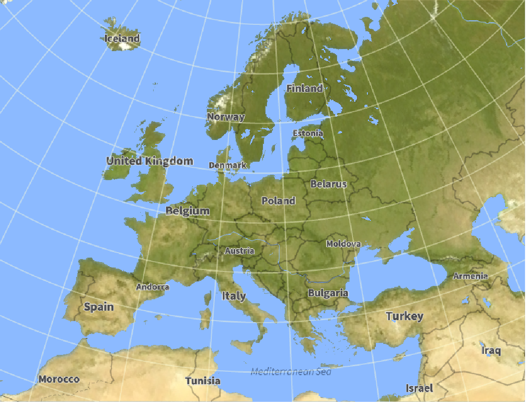
Because entity classes are taken as a collection of polygons, showing a map of Europe includes internal national boundaries:
GeoGraphics[{GeoStyling[GrayLevel[.7]], EdgeForm[Red], Polygon[EntityClass["Country", "Europe"]]}, GeoBackground -> "Plain"]Use the "GeographicRegion" entity for Europe instead:
GeoGraphics[{GeoStyling[GrayLevel[.7]], EdgeForm[Red], Polygon[Entity["GeographicRegion", "Europe"]]}, GeoBackground -> "Plain"]Interactive Examples (1)
Extract location and times from a time series object representing a short stroll and then compute distance traveled and average speed:
ts = TemporalData[TimeSeries, {{{GeoPosition[{38.610888, -90.253012, 150.16666666666666}],
    GeoPosition[{38.610849, -90.252845, 150.14285714285714}],
    GeoPosition[{38.61092, -90.252744, 150.125}],
    GeoPosition[{38.610939, -90.252637, 150.111 ... 365*^9,
     3.59925186864900000000000090949470177292823791504`24.573836111883047*^9,
     3.59925187461800000000005184119800105690956115723`24.345914052163195*^9}}}, 1,
  {"Discrete", 1}, {"Discrete", 1}, 1, {ValueDimensions -> 1}}, True, 10.];
x = ts["Values"];
dist = Prepend[
	UnitConvert[GeoDistance@@#& /@ Partition[x, 2, 1], "Miles"], Quantity[0, "Miles"]
	];
dt = Quantity[-#, "Seconds"]& /@ Subtract@@@Partition[ts["Times"], 2, 1];
time = Prepend[Accumulate[dt], Quantity[0, "Seconds"]];
speed = Prepend[
	UnitConvert[Rest[dist] / dt, "MilesPerHour"],
	Quantity[0, "MilesPerHour"]
	];
cornerPoints = Point[GeoPosition[(Transpose[{Min@#, Max@#}& /@ Transpose[x[[ ;; , 1, ;; 2]]]] + .001{{-1, -1}, {1, 1}})]];Manipulate[
With[{i = LengthWhile[QuantityMagnitude[time], # <= t&]},
GeoGraphics[{
cornerPoints,
Line[GeoPosition[If[Length[#] === 1, {#[[1]], #[[1]]}, #]&@x[[ ;; i, 1, ;; 2]]]]
},
PlotLabel -> Grid[{
{Style["Speed: ", Black, Bold], Round[speed[[i]], .01]}, {Style["Distance traveled: ", Black, Bold], If[i == 1, Quantity[0, "Miles"], Round[Total[dist[[ ;; i - 1]]], .01]]}
}, Alignment -> {{Right, Left}}
]]
],
{{t, 0, "t"}, 0, Ceiling[QuantityMagnitude[Last[time]]]}, SaveDefinitions -> True]Neat Examples (6)
Drape the African nations in their national flags:
flags = EntityValue[EntityClass["Country", "Africa"], {"Entity", "FlagImage"}];Place flag images on countries and use the country names as tooltips:
GeoGraphics[{EdgeForm[Black], {GeoStyling[{"Image", #2}], Tooltip[Polygon[#1], CommonName[#1]]}&@@@flags}, GeoBackground -> "StreetMapNoLabels"]Use flag images annotated with country names as tooltips:
GeoGraphics[{GeoStyling["OutlineMap"], Tooltip[Polygon[#1], Labeled[#1, #2]]&@@@flags}, GeoBackground -> "StreetMapNoLabels"]Find the graph of neighboring European countries:
countries = EntityList[EntityClass["Country", "EuropeSovereign"]];graph = Graph[countries, Flatten[EntityValue[countries, EntityFunction[e, Thread[e -> Intersection[e["BorderingCountries"], countries]]]]]]coloring = FindVertexColoring[graph, {RGBColor[0.29, 0.588, 0.612], RGBColor[0.886243, 0.527215, 0.0910023], RGBColor[0.613966, 0.37652, 0.585084], RGBColor[0.521981, 0.66, 0.0942065]}];GeoGraphics[Transpose[{GeoStyling /@ coloring, Polygon /@ countries}], GeoBackground -> None]Show national flags of some countries and speak their names when clicked:
GeoGraphics[{GeoStyling[{"Image", CountryData[#, "Flag"]}], EventHandler[Polygon[Entity["Country", #]], {"MouseClicked" :> Speak[#]}]}& /@ {"France", "Germany", "Italy", "Spain"}]Transform country polygons into shapes with rounded borders using filled B‐spline curves:
roundify[Polygon[l_], δ_] := FilledCurve[BSplineCurve[GeoPosition[#], SplineClosed -> True]]&  /@
Select[(DeleteDuplicates[Round[#, δ]]& /@ Level[l, {-3}]), Length[#] > 3&](color[#] = RandomColor[])& /@ (countries = CountryData["Europe"]);Display countries as "puzzle pieces":
GeoGraphics[
	{GeoStyling["OutlineMap", Directive[Opacity[0.4], EdgeForm[Black], color[#]]], Tooltip[roundify[CountryData[#, "FullPolygon"], 1.5], CommonName[#]]}& /@ countries,
	GeoBackground -> "ReliefMap", GeoRange -> {{34, 72}, {-25, 40}}, GeoRangePadding -> Full]
Retrieve names, locations, and yields of all nuclear explosions detonated by the United States:
data = EntityValue[EntityClass["NuclearExplosion", {"DetonationCountry", "UnitedStates"}], {"Name", "Yield", "Position"}];GeoGraphics[{Red, PointSize[Medium], Tooltip[Point[#3], Column[{#1, #2}]]&@@@data}, GeoRange -> "World"]Paint a purple spiral on France:
poly = MovingAverage[Join[#, Take[#, 10]]&[CountryData[Entity["Country", "France"], "Polygon"][[1, 1, 1]]], 11];{center, λ, δ} = {Mean[poly], Length[poly], 1 / 10};GeoGraphics[{GeoStyling["OutlineMap", Directive[Purple, Opacity[0.8]]], FilledCurve[Table[Line[GeoPosition[MapIndexed[(center + (s + 2 δ #2[[1]] / λ) (#1 - center))&, poly]]], {s, 0, 1 - 2 δ, δ}]]}]Text
Wolfram Research (2014), GeoGraphics, Wolfram Language function, https://reference.wolfram.com/language/ref/GeoGraphics.html (updated 2025).
CMS
Wolfram Language. 2014. "GeoGraphics." Wolfram Language & System Documentation Center. Wolfram Research. Last Modified 2025. https://reference.wolfram.com/language/ref/GeoGraphics.html.
APA
Wolfram Language. (2014). GeoGraphics. Wolfram Language & System Documentation Center. Retrieved from https://reference.wolfram.com/language/ref/GeoGraphics.html