


MeshConnectivityGraph
MeshConnectivityGraph[mr,0]
gives a graph of points connected by lines.
MeshConnectivityGraph[mr,d]
gives a graph between cells of dimension d that share a cell of dimension d-1.
MeshConnectivityGraph[mr,{d,e},r]
gives a graph from cells of dimension d to cells of dimension e that share a cell of dimension r.
Details and Options
- MeshConnectivityGraph is also known as mesh adjacency graph and mesh incidence graph.
- Typical uses include getting cell adjacencies and topological information in a mesh.
- A vertex {d,i} in the connectivity graph corresponds to the cell cd,i with dimension d and index i in the mesh mr.
- An undirected edge in MeshConnectivityGraph[mr,d]connects two vertices {d,i} and {d,j} whenever the cells cd,i and cd,j both have a common subcell of dimension d-1. For d=0, the common subcell has dimension 1.
- Common cases for d are:
-
0 points that share a line 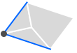
1 lines that share a point 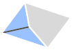
2 polygons that share an edge 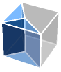
3 polyhedra that share a polygon - In MeshConnectivityGraph[mr,{d,e},r], a directed edge connects the vertex {d,i} to the vertex {e,j} whenever the cells cd,i and ce,j have a common cell of dimension r that is either a subset or a superset of cd,i and ce,j.
- MeshConnectivityGraph[mr] is effectively equivalent to MeshConnectivityGraph[mr,0].
- MeshConnectivityGraph[mr,d,r] is equivalent to the undirected graph of the graph MeshConnectivityGraph[mr,{d,d},r].
- MeshConnectivityGraph takes the same options as Graph with the following changes:
-
AnnotationRules Inherited
List of all options
Examples
open all close allBasic Examples (2)
Construct a connectivity graph between cells of dimension 0 in a mesh:
mesh = MengerMesh[2]Points are connected if they shared the same edges:
g = MeshConnectivityGraph[mesh, 0]Find a shortest path between two vertices of cell indices {0,1} and {0,96}:
FindShortestPath[g, {0, 1}, {0, 96}]HighlightGraph[g, PathGraph[%]]Get the connectivity matrix between faces of an icosahedron:
MeshConnectivityGraph[Icosahedron[], {2, 2}]AdjacencyMatrix[%]Scope (4)
MeshConnectivityGraph works on MeshRegion:
MeshConnectivityGraph[[image], 0]MeshConnectivityGraph[[image], 0]MeshConnectivityGraph[Rectangle[], 0]MeshConnectivityGraph works on all dimensions:
Table[MeshConnectivityGraph[[image], d], {d, {0, 1, 2, 3}}]Construct a connectivity graph between cells of dimension 0 in a mesh:
MeshConnectivityGraph[[image], 0]Between cells of dimension 0 and 1:
MeshConnectivityGraph[[image], {0, 1}]Between cells of dimension 0 and 0 sharing the same face:
MeshConnectivityGraph[[image], {0, 0}, 2]By default, AnnotationRulesInherited annotations are preserved:
MeshConnectivityGraph[Triangle[], {0, 1}]VertexList[%]With the setting AnnotationRulesNone, annotations are not preserved and the graph is indexed:
MeshConnectivityGraph[Triangle[], 0, AnnotationRules -> None]VertexList[%]Options (81)
AnnotationRules (4)
Specify an annotation for vertices:
MeshConnectivityGraph[Triangle[], 0, AnnotationRules -> {1 -> {VertexLabels -> "hello"}}]MeshConnectivityGraph[Triangle[], 0, AnnotationRules -> {12 -> {EdgeLabels -> "hello"}}]MeshConnectivityGraph[Triangle[], 0, AnnotationRules -> {"GraphProperties" -> {"Message" -> "hello"}}]AnnotationValue[%, "Message"]With the setting AnnotationRulesNone, annotations are not preserved and the graph is indexed:
MeshConnectivityGraph[Triangle[], 0, AnnotationRules -> None]VertexList[%]DirectedEdges (1)
By default, a directed path is generated when computing connectivity between cells of different dimensions:
MeshConnectivityGraph[Triangle[], {0, 1}]Use DirectedEdges->False to interpret rules as undirected edges:
MeshConnectivityGraph[Triangle[], {0, 1}, DirectedEdges -> False]EdgeLabels (7)
MeshConnectivityGraph[Triangle[], 0, EdgeLabels -> {{0, 1}{0, 2} -> "Hello"}]el = EdgeList[MeshConnectivityGraph[Triangle[], 0]];MeshConnectivityGraph[Triangle[], 0, EdgeLabels -> Table[el[[i]] -> Subscript["e", i], {i, Length[el]}]]Use any expression as a label:
MeshConnectivityGraph[Triangle[], 0, EdgeLabels -> {{0, 1}{0, 2} -> [image], {0, 2}{0, 3} -> [image], {0, 3}{0, 1} -> [image]}]Use Placed with symbolic locations to control label placement along an edge:
Table[MeshConnectivityGraph[Triangle[], 0, EdgeLabels -> {{0, 1}{0, 2} -> Placed["■■■", p]}, PlotLabel -> p], {p, {"Start", "Middle", "End"}}]Use explicit coordinates to place labels:
Table[MeshConnectivityGraph[Triangle[], 0, EdgeLabels -> {{0, 2}{0, 3} -> Placed["■■■", p]}, PlotLabel -> p, BaselinePosition -> Bottom], {p, {0, 1 / 4, 1 / 3}}]Vary positions within the label:
Table[MeshConnectivityGraph[Triangle[], 0, EdgeLabels -> {{0, 1}{0, 2} -> Placed["■■■", {1 / 2, p}]}, PlotLabel -> p, BaselinePosition -> Bottom], {p, {{0, 0}, {1 / 2, 1 / 2}, {1, 1}}}]MeshConnectivityGraph[Triangle[], 0, EdgeLabels -> {{0, 3}{0, 1} -> Placed[{"lbl1", "lbl2"}, {"Start", "End"}]}]MeshConnectivityGraph[Triangle[], 0, EdgeLabels -> {{0, 3}{0, 1} -> Placed[{"lbl1", "lbl2", "lbl3"}, {"Start", "Middle", "End"}]}]Use automatic labeling by values through Tooltip and StatusArea:
MeshConnectivityGraph[Triangle[], 0, EdgeLabels -> Placed["Name", Tooltip]]MeshConnectivityGraph[Triangle[], 0, EdgeLabels -> Placed["Name", StatusArea]]EdgeShapeFunction (6)
Get a list of built-in settings for EdgeShapeFunction:
ResourceData["EdgeShapeFunction"]Undirected edges including the basic line:
MeshConnectivityGraph[Triangle[], 0, EdgeShapeFunction -> "Line"]Lines with different glyphs on the edges:
Table[MeshConnectivityGraph[Triangle[], 0, EdgeShapeFunction -> {{ef, "ArrowSize" -> 0.1}}, PlotLabel -> ef], {ef, {"BoxLine", "DiamondLine", "DotLine"}}]Directed edges including solid arrows:
Table[MeshConnectivityGraph[Triangle[], 0, EdgeShapeFunction -> {{ef, "ArrowSize" -> 0.1}}, PlotLabel -> ef], {ef, ResourceData["EdgeShapeFunction", "FilledArrow"]}]Table[MeshConnectivityGraph[Triangle[], 0, EdgeShapeFunction -> {{ef, "ArrowSize" -> 0.1}}, PlotLabel -> ef], {ef, ResourceData["EdgeShapeFunction", "UnfilledArrow"]}]Table[MeshConnectivityGraph[Triangle[], 0, EdgeShapeFunction -> {{ef, "ArrowSize" -> 0.1}}, PlotLabel -> ef], {ef, ResourceData["EdgeShapeFunction", "CarvedArrow"]}]Specify an edge function for an individual edge:
MeshConnectivityGraph[Triangle[], 0, EdgeShapeFunction -> {{0, 1}{0, 2} -> "DotLine"}]Combine with a different default edge function:
MeshConnectivityGraph[Triangle[], 0, EdgeShapeFunction -> {{0, 1}{0, 2} -> "BoxLine", "DotLine"}]Draw edges by running a program:
ef[pts_List, e_] :=
Block[{s = 0.015, g = [image]}, {Arrowheads[{{s, 0.33, g}, {s, 0.67, g}}], Arrow[pts]}]MeshConnectivityGraph[Triangle[], 0, EdgeShapeFunction -> ef]EdgeShapeFunction can be combined with EdgeStyle:
MeshConnectivityGraph[Triangle[], 0, EdgeStyle -> Blue, EdgeShapeFunction -> (Line[#1]&)]EdgeShapeFunction has higher priority than EdgeStyle:
MeshConnectivityGraph[Triangle[], 0, EdgeStyle -> Blue, EdgeShapeFunction -> ({Red, Line[#1]}&)]EdgeStyle (2)
EdgeWeight (2)
Specify a weight for all edges:
MeshConnectivityGraph[Triangle[], 0, EdgeWeight -> RandomInteger[5, 3]]WeightedAdjacencyMatrix[%]//MatrixFormUse any numeric expression as a weight:
MeshConnectivityGraph[Triangle[], 0, EdgeWeight -> {a, b, c}]WeightedAdjacencyMatrix[%]//MatrixFormGraphHighlight (3)
MeshConnectivityGraph[Triangle[], 0, VertexSize -> Tiny, GraphHighlight -> {{0, 1}}]Highlight the edge {0,2}{0,3}:
MeshConnectivityGraph[Triangle[], 0, VertexSize -> Tiny, GraphHighlight -> {{0, 2}{0, 3}}]MeshConnectivityGraph[Triangle[], 0, VertexSize -> Tiny, GraphHighlight -> {{0, 1}, {0, 2}, {0, 1}{0, 2}}]GraphHighlightStyle (2)
Get a list of built-in settings for GraphHighlightStyle:
ResourceData["GraphHighlightStyle"]Use built-in settings for GraphHighlightStyle:
MeshConnectivityGraph[Triangle[], 0, GraphHighlight -> {{0, 1}, {0, 2}{0, 3}}, VertexSize -> Small, GraphHighlightStyle -> #, PlotLabel -> #]& /@ Select[ResourceData["GraphHighlightStyle"], # =!= Automatic&]GraphLayout (5)
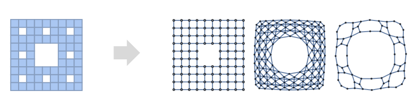
By default, the layout is chosen automatically:
MeshConnectivityGraph[MengerMesh[2], 0, GraphLayout -> Automatic]Specify layouts on special curves:
Table[MeshConnectivityGraph[MengerMesh[1], 0, GraphLayout -> l, PlotLabel -> l], {l, {"CircularEmbedding", "SpiralEmbedding"}}]Specify layouts that satisfy optimality criteria:
Table[MeshConnectivityGraph[MengerMesh[2], 0, GraphLayout -> l, PlotLabel -> l], {l, {"SpringEmbedding", "SpringElectricalEmbedding", "HighDimensionalEmbedding"}}]VertexCoordinates overrides GraphLayout coordinates:
{MeshConnectivityGraph[Triangle[], 0, GraphLayout -> "SpringElectricalEmbedding"],
	MeshConnectivityGraph[Triangle[], 0, GraphLayout -> "SpringElectricalEmbedding", VertexCoordinates -> Table[{i, i}, {i, 0, 2}]]}
Use AbsoluteOptions to extract VertexCoordinates computed using a layout algorithm:
MeshConnectivityGraph[Triangle[], 0]AbsoluteOptions[%, VertexCoordinates]PlotTheme (4)
Base Themes (2)
VertexCoordinates (2)
By default, any vertex coordinates are computed automatically:
MeshConnectivityGraph[Triangle[], 0]Extract the resulting vertex coordinates using AbsoluteOptions:
AbsoluteOptions[%, VertexCoordinates]Specify a layout function along an ellipse:
ellipseLayout[n_, {a_, b_}] := Table[{a Cos[2Pi / n u], b Sin[2Pi / n u]}, {u, 1, n}]Graphics[Point[ellipseLayout[16, {2, 1}]]]Use it to generate vertex coordinates for a graph:
MeshConnectivityGraph[MengerMesh[1], 0, VertexCoordinates -> ellipseLayout[16, {2, 1}]]VertexLabels (13)
MeshConnectivityGraph[Triangle[], 0, VertexLabels -> "Name"]MeshConnectivityGraph[Triangle[], 0, VertexLabels -> {{0, 1} -> "one"}]MeshConnectivityGraph[Triangle[], 0, VertexLabels -> Table[{0, i} -> Subscript[v, i], {i, 3}]]Use any expression as a label:
MeshConnectivityGraph[Triangle[], 0, VertexLabels -> {{0, 1} -> **[image]**, {0, 2} -> [image], {0, 3} -> [image]}]Use Placed with symbolic locations to control label placement, including outside positions:
Table[MeshConnectivityGraph[Triangle[], 0, VertexSize -> 0.1, VertexShapeFunction -> "Square", VertexLabels -> Table[{0, i} -> Placed["■■■", p], {i, 3}], PlotLabel -> p, ImagePadding -> 20], {p, {Before, After, Below, Above}}]Symbolic outside corner positions:
pl = {{Before, Below}, {After, Below}, {Before, Above}, {After, Above}};Table[MeshConnectivityGraph[Triangle[], 0, VertexSize -> 0.1, VertexShapeFunction -> "Square", ImagePadding -> 20, VertexLabels -> Table[{0, i} -> Placed["■■■", p], {i, 3}], PlotLabel -> p], {p, pl}]Table[MeshConnectivityGraph[Triangle[], 03, VertexSize -> 0.25, VertexLabels -> Table[{0, i} -> Placed["■■■", p], {i, 3}], VertexShapeFunction -> "Square", PlotLabel -> p], {p, {Left, Top, Right, Bottom}}]Symbolic inside corner positions:
pl = {{Left, Bottom}, {Right, Bottom}, {Left, Top}, {Right, Top}};Table[MeshConnectivityGraph[Triangle[], 0, VertexSize -> 0.25, VertexShapeFunction -> "Square", VertexLabels -> Table[{0, i} -> Placed["■■■", p], {i, 3}], PlotLabel -> p], {p, pl}]Use explicit coordinates to place the center of labels:
Table[MeshConnectivityGraph[Triangle[], 0, VertexSize -> 0.25, VertexShapeFunction -> "Square", VertexLabels -> Table[{0, i} -> Placed[[image], p], {i, 3}], PlotLabel -> p, BaselinePosition -> Bottom], {p, {{0, 0}, {1 / 2, 1 / 2}, {1, 1}}}]Place all labels at the upper-right corner of the vertex and vary the coordinates within the label:
Table[MeshConnectivityGraph[Triangle[], 0, VertexSize -> 0.35, VertexShapeFunction -> "Square", VertexLabels -> Table[{0, i} -> Placed[[image], {{1, 1}, p}], {i, 3}], PlotLabel -> p, BaselinePosition -> Bottom], {p, {{0, 0}, {1 / 2, 1 / 2}, {1, 1}}}]MeshConnectivityGraph[Triangle[], 0, VertexLabels -> {{0, 1} -> Placed[{"lbl1", "lbl2"}, {Above, Below}]}]Any number of labels can be used:
MeshConnectivityGraph[Triangle[], 0, VertexLabels -> {{0, 1} -> Placed[{"lbl1", "lbl2", "lbl3", "lbl4"}, {Above, After, Below, Before}]}]Use the argument to Placed to control formatting including Tooltip:
MeshConnectivityGraph[Triangle[], 0, VertexLabels -> Placed["Name", Tooltip]]Or StatusArea:
MeshConnectivityGraph[Triangle[], 0, VertexLabels -> Placed["Name", StatusArea]]Use more elaborate formatting functions:
rotateLabel[lab_] := Rotate[lab, 45Degree]MeshConnectivityGraph[Triangle[], 0, VertexLabels -> Table[{0, i} -> Placed["xxx", Below, rotateLabel], {i, 3}]]panelLabel[lab_] := Panel[lab, FrameMargins -> 0, Background -> Lighter[Yellow, 0.7]]MeshConnectivityGraph[Triangle[], 0, VertexLabels -> Table[{0, i} -> Placed["xxx", Center, panelLabel], {i, 3}]]hyperlinkLabel[lab_] := Hyperlink[lab, "http://www.wolfram.com"]MeshConnectivityGraph[Triangle[], 0, VertexLabels -> Table[{0, i} -> Placed["xxx", Center, hyperlinkLabel], {i, 3}]]VertexShape (5)
Use any Graphics, Image or Graphics3D as a vertex shape:
Table[MeshConnectivityGraph[Triangle[], 0, VertexShape -> s, VertexSize -> Medium], {s, {[image], [image], [image]}}]Specify vertex shapes for individual vertices:
MeshConnectivityGraph[Triangle[], 0, VertexShape -> {{0, 2} -> [image]}, VertexSize -> Small]VertexShape can be combined with VertexSize:
Table[MeshConnectivityGraph[Triangle[], 0, VertexSize -> s, VertexShape -> [image], PlotLabel -> s], {s, {Small, Large}}]VertexShape is not affected by VertexStyle:
MeshConnectivityGraph[Triangle[], 0, VertexSize -> 0.2, VertexShape -> [image], VertexStyle -> Blue]VertexShapeFunction has higher priority than VertexShape:
MeshConnectivityGraph[Triangle[], 0, VertexSize -> 0.1, VertexShapeFunction -> "Square", VertexShape -> [image]]VertexShapeFunction (10)
Get a list of built-in collections for VertexShapeFunction:
ResourceData["VertexShapeFunction"]Use built-in settings for VertexShapeFunction in the "Basic" collection:
ResourceData["VertexShapeFunction", "Basic"]Table[MeshConnectivityGraph[Triangle[], 0, VertexShapeFunction -> vf, VertexSize -> 0.2, PlotLabel -> vf], {vf, {"Triangle", "Square", "Rectangle", "Pentagon", "Hexagon", "Octagon"}}]Table[MeshConnectivityGraph[Triangle[], 0, VertexShapeFunction -> vf, VertexSize -> 0.2, PlotLabel -> vf], {vf, {"DownTrapezoid", "UpTrapezoid", "Parallelogram", "FiveDown", "Circle", "Diamond", "Star", "Capsule"}}]Use built-in settings for VertexShapeFunction in the "Rounded" collection:
ResourceData["VertexShapeFunction", "Rounded"]Table[MeshConnectivityGraph[Triangle[], 0, VertexShapeFunction -> vf, VertexSize -> 0.2, PlotLabel -> vf], {vf, ResourceData["VertexShapeFunction", "Rounded"]}]Use built-in settings for VertexShapeFunction in the "Concave" collection:
ResourceData["VertexShapeFunction", "Concave"]Table[MeshConnectivityGraph[Triangle[], 0, VertexShapeFunction -> vf, VertexSize -> 0.2, PlotLabel -> vf], {vf, ResourceData["VertexShapeFunction", "Concave"]}]MeshConnectivityGraph[Triangle[], 0, VertexShapeFunction -> { {0, 1} -> "Square"}, VertexSize -> 0.2]Combine with a default vertex function:
MeshConnectivityGraph[Triangle[], 0, VertexShapeFunction -> { {0, 1} -> "Square", "Triangle"}, VertexSize -> 0.2]Draw vertices using a predefined graphic:
MeshConnectivityGraph[Triangle[], 0, VertexShapeFunction -> (Inset[[image], #]&)]Draw vertices by running a program:
vf[{xc_, yc_}, name_, {w_, h_}] :=
	Block[{xmin = xc - w, xmax = xc + w, ymin = yc - h, ymax = yc + h},
	Polygon[{{xmin, ymin}, {xmax, ymax}, {xmin, ymax}, {xmax, ymin}}]
];MeshConnectivityGraph[Triangle[], 0, VertexShapeFunction -> vf, VertexSize -> 0.2]VertexShapeFunction can be combined with VertexStyle:
vf1[{xc_, yc_}, name_, {w_, h_}] := Rectangle[{xc - w, yc - h}, {xc + w, yc + h}]MeshConnectivityGraph[Triangle[], 0, VertexSize -> 0.2, VertexStyle -> Blue, VertexShapeFunction -> vf1]VertexShapeFunction has higher priority than VertexStyle:
vf2[{xc_, yc_}, name_, {w_, h_}] := {Red, Rectangle[{xc - w, yc - h}, {xc + w, yc + h}]}MeshConnectivityGraph[Triangle[], 0, VertexSize -> 0.2, VertexStyle -> Blue, VertexShapeFunction -> vf2]VertexShapeFunction can be combined with VertexSize:
MeshConnectivityGraph[Triangle[], 0, VertexShapeFunction -> "Star", VertexSize -> {{0, 1} -> Small, Medium}]VertexShapeFunction has higher priority than VertexShape:
MeshConnectivityGraph[Triangle[], 0, VertexSize -> 0.3, VertexShapeFunction -> "Star", VertexShape -> [image]]VertexSize (8)
By default, the size of vertices is computed automatically:
MeshConnectivityGraph[Triangle[], 0, VertexSize -> Automatic]Specify the size of all vertices using symbolic vertex size:
Table[MeshConnectivityGraph[Triangle[], 0, VertexSize -> s, PlotLabel -> s], {s, {Tiny, Small, Medium, Large}}]Use a fraction of the minimum distance between vertex coordinates:
Table[MeshConnectivityGraph[Triangle[], 0, VertexSize -> s, PlotLabel -> s], {s, 0.1, 1, 0.3}]Use a fraction of the overall diagonal for all vertex coordinates:
Table[MeshConnectivityGraph[Triangle[], 0, VertexSize -> {"Scaled", s}, PlotLabel -> {"Scaled", s}], {s, 0.1, 1, 0.3}]Specify size in both the ![]() and
and ![]() directions:
directions:
Table[MeshConnectivityGraph[Triangle[], 0, VertexSize -> s, PlotLabel -> s], {s, {{0.1, 0.2}, {0.2, 0.1}}}]Specify the size for individual vertices:
MeshConnectivityGraph[Triangle[], 0, VertexSize -> {{0, 1} -> 0.2, {0, 2} -> 0.3}]VertexSize can be combined with VertexShapeFunction:
Table[MeshConnectivityGraph[Triangle[], 0, VertexSize -> s, VertexShapeFunction -> "Square", PlotLabel -> s], {s, {0.05, 0.1, 0.2}}]VertexSize can be combined with VertexShape:
Table[MeshConnectivityGraph[Triangle[], 0, VertexSize -> s, VertexShape -> [image], PlotLabel -> s], {s, {0.1, 0.2, 0.4}}]VertexStyle (5)
Table[MeshConnectivityGraph[Triangle[], 0, VertexStyle -> style, VertexSize -> 0.3], {style, {Yellow, EdgeForm@Dashed}}]MeshConnectivityGraph[Triangle[], 0, VertexStyle -> {{0, 1} -> Blue, {0, 2} -> Red}, VertexSize -> 0.2]VertexShapeFunction can be combined with VertexStyle:
vf1[{xc_, yc_}, name_, {w_, h_}] := Rectangle[{xc - w, yc - h}, {xc + w, yc + h}]MeshConnectivityGraph[Triangle[], 0, VertexSize -> 0.2, VertexStyle -> Blue, VertexShapeFunction -> vf1]VertexShapeFunction has higher priority than VertexStyle:
vf2[{xc_, yc_}, name_, {w_, h_}] := {Red, Rectangle[{xc - w, yc - h}, {xc + w, yc + h}]}MeshConnectivityGraph[Triangle[], 0, VertexSize -> 0.2, VertexStyle -> Blue, VertexShapeFunction -> vf2]VertexStyle can be combined with BaseStyle:
MeshConnectivityGraph[Triangle[], 0, VertexStyle -> LightBlue, BaseStyle -> EdgeForm[Dotted], VertexSize -> 0.2]VertexStyle has higher priority than BaseStyle:
MeshConnectivityGraph[Triangle[], 0, VertexStyle -> LightBlue, BaseStyle -> Gray, VertexSize -> 0.2]VertexShape is not affected by VertexStyle:
MeshConnectivityGraph[Triangle[], 0, VertexSize -> 0.2, VertexShape -> [image], VertexStyle -> Blue]VertexWeight (2)
Set the weight for all vertices:
MeshConnectivityGraph[Triangle[], 0, VertexWeight -> {2, 3, 4}]AnnotationValue[{%, {0, 1}}, VertexWeight]Use any numeric expression as a weight:
MeshConnectivityGraph[Triangle[], 0, VertexWeight -> {a, b, c}]AnnotationValue[{%, {0, 1}}, VertexWeight]Applications (10)
Basic Applications (5)
mesh = [image];MeshConnectivityGraph[mesh, {0, 0}, #]& /@ {0, 1, 2}Point to edge sharing the same face:
MeshConnectivityGraph[mesh, {0, 1}, 2, VertexLabels -> Automatic]mesh = [image];MeshConnectivityGraph[mesh, {0, 0}, #]& /@ {0, 1, 2}Point to edge sharing the same face:
MeshConnectivityGraph[mesh, {0, 1}, 2]Menger mesh connectivity graph:
mesh = MengerMesh[2]MeshConnectivityGraph[mesh, {0, 0}, #]& /@ {0, 1, 2}Point to edge sharing the same face:
MeshConnectivityGraph[mesh, {0, 1}, 2]3D boundary mesh connectivity graph:
mesh = [image];MeshConnectivityGraph[mesh, {0, 0}, #]& /@ {0, 1, 2}Point to edge sharing the same face:
MeshConnectivityGraph[mesh, {0, 1}, 2]Get the face adjacency of a Voronoi mesh:
pts = RandomReal[1, {10, 2}];mesh = VoronoiMesh[pts]centroids = RegionCentroid /@ MeshPrimitives[mesh, 2];Show[{mesh, MeshConnectivityGraph[mesh, 2, VertexCoordinates -> centroids ]}]Adjacency Queries (1)
Polyhedra Operations (1)
Use MeshConnectivityGraph to compute the DualPolyhedron of a cuboid:
cube = [image];Compute the connectivity graph between points and faces:
g = MeshConnectivityGraph[cube, {0, 2}]Get the adjacent faces for each point:
mat = AdjacencyMatrix[g];
faces  = Cases[mat["AdjacencyLists"] - MeshCellCount[cube, 0], Except[{}]]
Compute the coordinates of the dual:
pts = MeshCoordinates[cube];
fs  = And@@@ MeshCells[cube, 2];
coords = Table[Mean[pts[[i]]], {i, fs}]
Construct the dual of the cube:
dual = Polyhedron[coords, faces]Graphics3D[{Opacity[0.2], cube, dual}]Topological Operations (3)
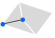
Use MeshConnectivityGraph to test whether a mesh is connected:
ConnectedMeshQ[mesh_] := ConnectedGraphQ[ MeshConnectivityGraph[mesh, 0, RegionDimension[mesh]]]Table[ConnectedMeshQ[i], {i, {[image], [image], [image], [image]}}]Use MeshConnectivityGraph to compute ConnectedMeshComponents:
mesh = [image];Connected components of a mesh connectivity graph:
com = ConnectedComponents[MeshConnectivityGraph[mesh, 0, 2, AnnotationRules -> None]]Group the mesh cells to different mesh connected components:
belong[a_, b_] := Length[Intersection[a, b]] == Length[a]cells = MeshCells[mesh, 2];
res = Flatten@Table[Position[belong[i, #]& /@ com, True], {i, cells[[All, 1]]}];groups = Gather[Thread[List[cells, res]], Last[#1] == Last[#2]&]Get mesh connected components:
Table[MeshRegion[MeshCoordinates[mesh], groups[[i]][[All, 1]]], {i, Length[com]}]![]() -skeleton graph of Platonic solids:
-skeleton graph of Platonic solids:
Table[MeshConnectivityGraph[reg, 0], {reg, {[image], [image], [image], [image], [image]}}]Properties & Relations (3)
The cell of index {d,k} corresponds to the vertex ![]() :
:
mesh = MeshRegion[{{0, 0}, {1, 0}, {2, 1 / 2}, {2, -1 / 2}}, {Line[{1, 2}], Line[{2, 3}], Line[{3, 4}], Line[{4, 2}]}]MeshConnectivityGraph[mesh, 1, VertexLabels -> "Name"]MeshConnectivityGraph between cells of different dimensions is a directed bipartite graph:
mesh = MeshRegion[{{0, 0, 0}, {2, 0, 0}, {2, 2, 0}, {0, 2, 0}, {1, 1, 2}}, {Tetrahedron[{1, 2, 3, 5}], Tetrahedron[{1, 3, 4, 5}]}]MeshConnectivityGraph[mesh, {1, 2}]BipartiteGraphQ[%]The AdjacencyMatrix of a mesh connectivity graph between cells of the same dimension is symmetric:
mesh = MeshRegion[{{0, 0, 0}, {2, 0, 0}, {2, 2, 0}, {0, 2, 0}, {1, 1, 2}}, {Tetrahedron[{1, 2, 3, 5}], Tetrahedron[{1, 3, 4, 5}]}]AdjacencyMatrix[MeshConnectivityGraph[mesh, {1, 1}]]SymmetricMatrixQ[%]Text
Wolfram Research (2020), MeshConnectivityGraph, Wolfram Language function, https://reference.wolfram.com/language/ref/MeshConnectivityGraph.html.
CMS
Wolfram Language. 2020. "MeshConnectivityGraph." Wolfram Language & System Documentation Center. Wolfram Research. https://reference.wolfram.com/language/ref/MeshConnectivityGraph.html.
APA
Wolfram Language. (2020). MeshConnectivityGraph. Wolfram Language & System Documentation Center. Retrieved from https://reference.wolfram.com/language/ref/MeshConnectivityGraph.html