



NMinimize
更多信息和选项
- NMinimize 亦称为全局优化 (GO).
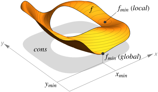
- NMinimize 总是尝试求给定约束条件限制下 f 的全局最小值.
- NMinimize 通常用于求给定约束条件下可能的最小值. 在不同的领域,这可能被称为最佳策略、最佳方案、最佳配置等.
- NMinimize 返回形如 {fmin,{x->xmin,y->ymin,…}} 的列表.
- 如果 f 和 cons 是线性的或凸的,NMinimize 给出的结果将是实数和整数值上的全局最小值;否则,有时结果可能只是局部最小值.
- 如果 NMinimize 发现无法满足约束条件,则会返回 {Infinity,{x->Indeterminate,…}}.
- NMinimize 支持一种建模语言,其中目标函数 f 和约束条件 cons 是用依赖于标量或向量变量的表达式给出的. f 和 cons 通常被解析为非常有效的形式,但只要 f 和 cons 中的项给出变量的数值结果,NMinimize 通常可以找到解.
- 约束条件 cons 可以是以下表达式的任意逻辑组合:
-
lhs==rhs 等式 lhs>rhs, lhs≥rhs, lhs<rhs, lhs≤rhs 不等式 (LessEqual、…) lhsrhs, lhsrhs, lhsrhs, lhsrhs 向量不等式 (VectorLessEqual、…) {x,y,…}∈rdom 区域或域的指定 - NMinimize[{f,cons},x∈rdom] 实际上等价于 NMinimize[{f,cons&&x∈rdom},x].
- 对于 x∈rdom,可用 Indexed[x,i] 来指代不同的坐标.
- 可能的域 rdom 包括:
-
Reals 实标量变量 Integers 整数标量变量 Vectors[n,dom]  中的向量变量
Matrices[{m,n},dom]  中的矩阵变量
ℛ 限制在几何区域  中的向量变量
- 默认情况下,假定所有变量为实数.
- 可给出下列选项:
-
AccuracyGoal Automatic 追求多少位的准确度 EvaluationMonitor None 计算 f 时要计算的表达式 MaxIterations Automatic 使用的最大迭代次数 Method Automatic 使用的方法 PrecisionGoal Automatic 追求多少位的精度 StepMonitor None 每次迭代时要计算的表达式 WorkingPrecision MachinePrecision 内部计算使用的精度 - AccuracyGoal 和 PrecisionGoal 的设置指定了搜索最小值所在位置(最小化点)和函数的最小值时应使用的位数.
- NMinimize 会持续运行,直到 AccuracyGoal 或 PrecisionGoal 指定的目标实现为止.
- NMinimize 的方法分为两类. 第一类方法利用问题的属性,因此当方法收敛时,找到的最小值保证是全局的. 第二类启发式方法使用的方法可能包括多个局部搜索,通常通过一些随机性进行调整以锁定全局最小值. 这些方法通常能找到全局最小值,但无法保证.
- 在收敛到解时确保可以给出全局最小值的方法包括:
-
"Convex" 只使用凸方法 "MOSEK" 对于凸问题,使用商用 MOSEK 库 "Gurobi" 对于凸问题,使用商用 Gurobi 库 "Xpress" 对于凸问题,使用商用 Xpress 库 - 启发式方法包括:
-
"NelderMead" Nelder 和 Mead 的单纯形法 "DifferentialEvolution" 使用差分进化 "SimulatedAnnealing" 使用模拟退火 "RandomSearch" 使用从多个随机起始点中找到的最佳局部最小值 "Couenne" 对非凸混合整数非线性问题使用 Couenne 库
范例
打开所有单元 关闭所有单元基本范例 (3)
NMinimize[x ^ 4 - 3x ^ 2 - x, x]x /. Last[NMinimize[x ^ 4 - 3x ^ 2 - x, x]]NMinimize[{x ^ 2 - (y - 1) ^ 2, x ^ 2 + y ^ 2 ≤ 4}, {x, y}]NMinimize[{E ^ (Sin[50 x]) + Sin[60 E ^ y] + Sin[70 Sin[x]] + Sin[Sin[80 y]] - Sin[10 (x + y)] + 1 / 4 (x ^ 2 + y ^ 2), x ^ 2 + y ^ 2 ≤ 1}, {x, y}]NMinimize[x + y, {x, y}∈Disk[]]Show[ContourPlot[x + y, {x, y}∈Disk[]], Graphics[{Red, PointSize[Large], Point[{x, y} /. Last[%]]}]]范围 (40)
基本用法 (12)


NMinimize[{x + 2y, x^2 + 2y^2 ≤ 3, x + y == 2, x ≥ 1}, {x, y}]可用 VectorGreaterEqual 表示几个线性不等式约束条件:
NMinimize[{x + y, VectorGreaterEqual[{{x + 2y, x}, {3, -1}}]}, {x, y}]用  v>=
 或 \[VectorGreaterEqual] 输入向量不等式符号 :
NMinimize[{x + y, {x + 2y, x}{3, -1}}, {x, y}]NMinimize[{x + y, x + 2y ≥ 3, x ≥ -1}, {x, y}]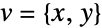
NMinimize[{{1, 1}.v, {{1, 2}, {1, 0}}.v{3, -1}}, v]
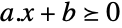

NMinimize[{{1, 1}.x, {{1, 2}, {1, 0}}.x + {-3, 1}0}, x]NMinimize[{{1, 1}.x, {{1, 2}, {1, 0}}.x{3, -1}}, x]如果想要避免  中不想要的逐项运算,可使用 Inactive[Plus]:
NMinimize[{{1, 1}.x, {{1, 2}, {1, 0}}.x + {-3, 1}0}, x]
parEqs = {a == {{1, 2}, {1, 0}}, b == {3, -1}};NMinimize[{{1, 1}.x, {parEqs, a.x + b0}}, x]VectorGreaterEqual 表示关于 "NonNegativeCone" 的锥不等式:
constraint = VectorGreaterEqual[{{{1, 2}, {1, 0}}.v, {3, -1}}, "NonNegativeCone"]如果想明确指定锥体的尺寸,可使用 {"NonNegativeCone",n}:
constraint = VectorGreaterEqual[{{{1, 2}, {1, 0}}.v, {3, -1}}, {"NonNegativeCone", 2}]NMinimize[{{1, 1}.v, constraint}, v]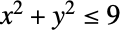

NMinimize[{x + y, x^2 + y^2 ≤ 9}, {x, y}]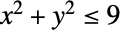
constraint = VectorGreaterEqual[{{x, y, 3}, 0}, {"NormCone", 3}]NMinimize[{x + y, constraint}, {x, y}]

{a, b} = {{{1, 1, 0}, {0, 1, 1}, {1, 1, 1}}, {2, 2, -1}};用 Indexed 访问向量变量的分量,如  :
NMinimize[{Total[x], a.xb, Indexed[x, 1] ≥ 1}, x]当向量变量不明确时,用 Vectors[n,dom] 指定维度和域:
NMinimize[{Indexed[x, {1}] + 2Indexed[x, {2}], (| | |
| --------------- | --------------- |
| Indexed[x, {1}] | 1 |
| 1 | Indexed[x, {2}] |)Underscript[, {"SemidefiniteCone", 2}]0}, x]
NMinimize[{Indexed[x, {1}] + Indexed[2x, {2}], (| | |
| --------------- | --------------- |
| Indexed[x, {1}] | 1 |
| 1 | Indexed[x, {2}] |)Underscript[, {"SemidefiniteCone", 2}]0}, x∈Vectors[2, Reals]]用 NonNegativeReals ( ) 指定非负约束条件:
NMinimize[{{1, 1}.x, {Indexed[x, {1}], Indexed[x, {2}], 1}Underscript[, {"NormCone", 3}]0}, x∈Vectors[2, NonNegativeReals]]
NMinimize[{{1, 1}.x, {Indexed[x, {1}], Indexed[x, {2}], 1}Underscript[, {"NormCone", 3}]0, x0}, x]用 NonPositiveReals ( ) 指定非正约束条件:
NMinimize[{-Total[v], {1, 2}.v-3}, v∈Vectors[2, NonPositiveReals]]NMinimize[{-Total[v], {1, 2}.v-3, v0}, v]也可以指定 Or 约束条件:
NMinimize[{x + y, x ^ 2 + y ^ 2 ≤ 1 || (x + 2) ^ 2 + (y + 2) ^ 2 ≤ 1}, {x, y}]//Quiet域约束条件 (4)
用 Integers 指定整数域约束条件:
NMinimize[{x + y, x + 2y ≥ 3, x ≥ -2}, {x∈Integers, y∈Integers}]用 Vectors[n,Integers] 指定向量变量的整数域约束条件:
NMinimize[{Total[x], a == {{1, 2}, {1, 0}}, b == {3, -2},
a.xb}, x∈Vectors[2, Integers]]用 NonNegativeIntegers ( ) 指定非负整数域约束条件:
NMinimize[{x + 2y, x^2 + 2y^2 ≤ 3, x + y == 2, x∈NonNegativeIntegers}, {x, y}]用 NonPositiveIntegers ( ) 指定非正整数域约束条件:
NMinimize[{-x + y, x + 2y ≥ 3, x∈NonPositiveIntegers}, {x, y}]区域约束条件 (5)
t = RotationTransform[{{0, 0, 1}, {1, 1, 1}}];
ℛ = TransformedRegion[Ellipsoid[{0, 0, 0}, {1, 2, 3}], t];NMinimize[z, {x, y, z}∈ℛ]Graphics3D[{{Opacity[0.5], Green, GeometricTransformation[Ellipsoid[{0, 0, 0}, {1, 2, 3}], t]}, {Red, PointSize[Large], Point[{x, y, z} /. Last[%]]}}]Subscript[ℛ, 1] = Disk[];
Subscript[ℛ, 2] = InfiniteLine[{{-2, 0}, {0, 2}}];NMinimize[EuclideanDistance[{x, y}, {u, v}], {{x, y}∈Subscript[ℛ, 1], {u, v}∈Subscript[ℛ, 2]}]Graphics[{{LightBlue, Subscript[ℛ, 1]}, {Green, Subscript[ℛ, 2]}, {Red, Point[{{x, y}, {u, v}} /. Last[%]]}}]
Subscript[ℛ, 1] = Triangle[{{0, 0}, {1, 0}, {0, 1}}];
Subscript[ℛ, 2] = Disk[{1, 1}, {2r, r}];NMinimize[{r, {x, y}∈Subscript[ℛ, 1] && {x, y}∈Subscript[ℛ, 2]}, {r, x, y}]Graphics[{{LightBlue, Subscript[ℛ, 1], Subscript[ℛ, 2]}, {Red, Point[{x, y}]}} /. Last[%]]Subscript[ℛ, 3] = Disk[{a, b}, r];NMinimize[{r, ({0, 0} | {1, 0} | {0, 1})∈Subscript[ℛ, 3]}, {a, b, r}]Graphics[{{LightBlue, Subscript[ℛ, 3]} /. %[[2]], {Red, Point[{{0, 0}, {1, 0}, {0, 1}}]}}]用 Circumsphere 直接给出同样的结果:
Circumsphere[{{0, 0}, {1, 0}, {0, 1}}]//N


ℛ = Sphere[];NMinimize[x.{1, 2, 3}, x∈ℛ]线性问题 (5)
NMinimize[{x + y, 3x + 2y ≥ 7 && x + 2y ≥ 6 && x ≥ 0 && y ≥ 0}, {x, y}]NMinimize[{x - y, x + y + z == 1 / 2, x - 2z == 1, 2x - y ≥ 1}, {x, y, z}]用 Equal 一次表示几个等式约束条件:
NMinimize[{x - y, {x + y, x - y} == {1 / 2, 1}}, {x, y}]NMinimize[{x - y, x + y == 1 / 2, x - y == 1}, {x, y}]用 VectorLessEqual 一次表示几个 LessEqual 不等式约束条件:
NMinimize[{x + y, VectorLessEqual[{{x - 2y, -x + y}, {3, 2}}]}, {x, y}]
 以紧凑格式输入向量不等式:
NMinimize[{x + y, {x - 2y, -x + y}{3, 2}}, {x, y}]NMinimize[{x + y, {x - 2y ≤ 3, -x + y ≤ 2}}, {x, y}]用 Interval 指定变量的范围:
NMinimize[{x + y, x + 2y ≥ 3}, {x∈Interval[{-1, 2}], y∈Interval[{-1, 1}]}]凸问题 (7)
用 "NonNegativeCone" 指定形如  的线性函数:
NMinimize[{Total[x],
	VectorGreaterEqual[{{{-1, -1 / 2}, {1, -1 / 2}, {0, 1}}.x, {-1 / 2, -1 / 2, -1 / 2}}, {"NonNegativeCone", 3}]}, x]
 以紧凑格式输入向量不等式:
NMinimize[{Total[x], {{-1, -(1/2)}, {1, -(1/2)}, {0, 1}}.x-(1/2)}, x]NMinimize[{(x - 1)^2 + y^2, x + y / 2 ≤ 1 / 2, x - y ≥ 0}, {x, y}]ContourPlot[(x - 1)^2 + y^2, {x, -1, 1}, {y, -1, 1 / 2}, ...]res = NMinimize[{(x - 1)^2 + y^2, x^2 + (y^2/2) ≤ (1/2), 2x^2 ≤ 3y}, {x, y}]Show[Plot3D[(x - 1)^2 + y^2, {x, -1, 1}, {y, 0, 1}, ...], Graphics3D[{Red, PointSize[0.03], Point[{x, y, (x - 1)^2 + y^2} /. res[[2]]]}]]Subscript[ℛ, 1] = Triangle[{{1, 1}, {2, 1}, {1, 2}}];
Subscript[ℛ, 2] = Disk[];NMinimize[EuclideanDistance[x, y], {x∈Subscript[ℛ, 1], y∈Subscript[ℛ, 2]}]Graphics[{{LightBlue, Subscript[ℛ, 1], Subscript[ℛ, 2]}, {Red, Point[{x, y}]}} /. %[[2]]]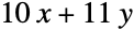

res = NMinimize[{10x + 11 y, (| | |
| - | - |
| x | 1 |
| 1 | y |)Underscript[, {"SemidefiniteCone", 2}]0}, {x, y}]Show[Plot3D[10x + 11y, {x, 0, 5}, {y, 0, 5}, ...], Graphics3D[{Red, PointSize[0.05], Point[{x, y, 10x + 11y} /. res[[2]]]}]]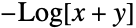
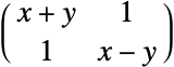

res = NMinimize[{-Log[x + y], (| | |
| ----- | ----- |
| x + y | 1 |
| 1 | x - y |)Underscript[, {"SemidefiniteCone", 2}]0, 1 ≤ x ≤ 10, -1 ≤ y ≤ 1}, {x, y}]Show[Plot3D[-Log[x + y], {x, 1, 10}, {y, -1, 1}, ...], Graphics3D[{Red, PointSize[0.05], Point[{x, y, -Log[x + y]} /. res[[2]]]}]]res = NMinimize[{(x - 2)^2 + (y - 1 / 2)^2, Inactive[Norm][{x, y}, 4] ≤ 1}, {x, y}]Show[Plot3D[(x - 2)^2 + (y - 1 / 2)^2, {x, -1, 1}, {y, -1, 1}, ...], Graphics3D[{PointSize[0.05], Point[{x, y, (x - 2)^2 + (y - (1/2))^2} /. res[[2]]]}]]可转化为凸问题的问题 (4)
NMinimize[{2w + 2h, h w == 1, h ≤ (1/2)w, h ≥ 0, w ≥ 0}, {h, w}]这个问题是对数-凸 (log-convex) 的,可以通过做一个变换 {hExp[],wExp[ ]} 并取对数得到凸问题来解决:
NMinimize[{Log[Exp[𝓌 + Log[2]] + Exp[𝒽 + Log[2]]], 𝒽 + 𝓌 == 0, 𝒽 - 𝓌 ≤ Log[1 / 2]}, {𝒽, 𝓌}]{Exp[First[%]], Thread[{h, w} -> Exp[{𝒽, 𝓌}] /. Last[%]]}最小化受不等式和范数约束条件限制的拟凸函数  . 目标函数是拟凸的,因为它是域上一个非负函数和一个非正函数的乘积:
NMinimize[{-x y, x ≥ 0, y ≥ 0, Norm[{x - 1, y - 2}] ≤ 1}, {x, y}]
pfun = ParametricConvexOptimization[0, {-x y ≤ α, x ≥ 0, y ≥ 0,
	Norm[{x - 1, y - 2}] ≤ 1}, {x, y}, α, "PrimalMinimizerRules"]
fun[α_ ? NumericQ] := -x * y /. pfun[α];
Plot[fun[α], {α, -4.68, 0}, PlotRange -> All]
pfun[-4.68]pfun[-4.69]
根据约束条件  最小化
 . 目标是非凸但可通过凸差函数
 表示,其中
 和
 为凸函数:
res = NMinimize[{x ^ 2 - y ^ 2, Norm[{x, y}] <= 2}, {x, y}]Show[Plot3D[x ^ 2 - y ^ 2, {x, -2, 2}, {y, -2, 2}, ...], Graphics3D[{PointSize[0.04], Point[{x, y, x ^ 2 - y ^ 2} /. res[[2]]]}]]根据约束条件  最小化
 . 约束条件
 为非凸但可通过凸差约束条件
 表示,其中
 和
 为凸函数:
res = NMinimize[{x ^ 2 + y, 1 <= Norm[{x, y}] <= 2}, {x, y}]Show[Plot3D[x ^ 2 + y, {x, -2, 2}, {y, -2, 2}, ...], Graphics3D[{PointSize[0.04], Point[{x, y, x ^ 2 + y} /. res[[2]]]}]]普通问题 (3)
res = NMinimize[{x + y, Sin[2x] + Cos[3y] ≤ 1, Norm[{x, y}] ≤ 2}, {x, y}]Show[Plot3D[x + y, {x, -2, 2}, {y, -2, 2}, ...], Graphics3D[{Blue, PointSize[0.03], Point[{x, y, x + y} /. res[[2]]]}]]res = NMinimize[{Sin[2x] + Cos[x], -2 ≤ x ≤ 3}, x]Plot[Sin[2x] + Cos[x], {x, -2, 3}, Epilog -> {...}]res = NMinimize[{Sin[x^2 + y], Sin[2x] + Cos[3y] ≤ 1, Norm[{x^2, y}] ≤ 2}, {x, y}]Show[Plot3D[Sin[x^2 + y], {x, -2, 2}, {y, -2, 2}, ...], Graphics3D[{Blue, PointSize[0.03], Point[{x, y, Sin[x^2 + y]} /. res[[2]]]}]]选项 (10)
AccuracyGoal 和 PrecisionGoal (2)

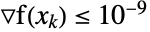
NMinimize[Sin[Tan[x] / 2], x, AccuracyGoal -> 9, PrecisionGoal -> 8]
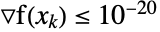
NMinimize[Sin[Tan[x] / 2], x, AccuracyGoal -> 20, PrecisionGoal -> 18]
设置一个较高的 WorkingPrecision ,使过程收敛:
NMinimize[Sin[Tan[x] / 2], x, AccuracyGoal -> 20, PrecisionGoal -> 18, WorkingPrecision -> 40]EvaluationMonitor (1)
f[x_, y_] := (x ^ 2 + y ^ 2 - 16) ^ 2;
{sol, pts} = Reap[
NMinimize[f[x, y], {{x, -5, 5}, {y, -5, 5}}, Method -> "DifferentialEvolution", EvaluationMonitor :> Sow[{x, y}]]];ContourPlot[f[x, y], {x, -5, 5}, {y, -5, 5}, ColorFunction -> (Hue[.6(1 - #1)]&),
Epilog -> Map[Point, Cases[First[pts], x_ /; Abs[f@@x - First[sol]] ≤ .05]], Contours -> 4Range[0, 10] ^ 2]Method (5)
NMinimize[{Sin[.4 x ^ 2] + .7Cos[.6 x] x, -9 < x < 9}, {x}, Method -> #]& /@ {"NelderMead", "DifferentialEvolution", "SimulatedAnnealing"}minSol = NMinimize[{Sin[.4 x ^ 2] + .7Cos[.6 x] x, -9 < x < 9}, {x}]minSol = NMinimize[{Sin[.4 x ^ 2] + .7Cos[.6 x] x, -9 < x < 9}, {x}, Method -> "Couenne"]Plot[Sin[.4 x ^ 2] + .7Cos[.6 x] x, {x, -9, 9}, Rule[...]]用 "Couenne" 法求包含多个局部最小值的函数的全局最小值
fun = E^Sin[50x] + Sin[60 E^y] + Sin[70 Sin[x]] + Sin[Sin[80 y]] - Sin[10 (x + y)] + (x^2 + y^2) / 4;
res = NMinimize[Evaluate[fun], {x, y}, Method -> "Couenne"]Show[Plot3D[fun, ...], Graphics3D[{...}]]当速度至关重要时,请使用方法 "NelderMead" 来求解有多个变量的问题:
n = 50;AbsoluteTiming[NMinimize[Sum[i * (x[i] - i) ^ 2 + Sin[x[i]], {i, 1, n}], Table[x[i], {i, 1, n}], Method -> "NelderMead"]]用 "Convex" 方法或 Except["Convex"] 指定是否应使用凸方法:
NMinimize[x^2 + y^2, {x + y == 1, x ^ 2 + 5y ^ 2 < 1}, {x, y}, Method -> #]& /@ {"Convex", Except["Convex"]}用 "Couenne" 方法或 Except["Couenne"] 选择或排除 Couenne 求解器:
NMinimize[Sin[x^2 + y^2], {x + y == 1, x ^ 2 + 5y ^ 2 < 1}, {x, y}, Method -> #]& /@ {"Couenne", Except["Couenne"]}StepMonitor (1)
在求经典的 Rosenbrock 函数最小值的过程中 NMinimize 采取的步骤:
pts = Reap[NMinimize[(1 - x) ^ 2 + 100(-x ^ 2 - y) ^ 2, {x, y},
	Method -> "NelderMead", StepMonitor :> Sow[{x, y}]]][[2, 1]];
pts = Join[{{-1.2, 1}}, pts];ContourPlot[(1 - x) ^ 2 + 100(-x ^ 2 - y) ^ 2, {x, -1.3, 1.5}, {y, -1.5, 1.4}, Epilog -> {Arrow[pts], Point[pts]}, Contours -> Table[10 ^ -i, {i, -2, 10}], ColorFunction -> (Hue[(Log[10, #] + 10) / 12]&), ColorFunctionScaling -> False]WorkingPrecision (1)
工作精度设为  时,AccuracyGoal 和 PrecisionGoal 默认值为
 :
NMinimize[Cos[x ^ 2 - 3 y] + Sin[x ^ 2 + y ^ 2], {x, y}, WorkingPrecision -> 20]应用 (19)
几何问题 (4)
求半径为 1、圆心为 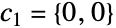 和
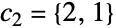 的两个圆盘之间的最小距离. 令
 为圆盘 1 上的一个点. 令
 为圆盘 2 上的一个点. 目标是最小化受约束条件
 限制的
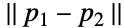 :
res = NMinimize[{Norm[p1 - p2], c2 == {2, 1}, Norm[p1] ≤ 1, Norm[p2 - c2] ≤ 1}, {p1∈Vectors[2, Reals], p2∈Vectors[2, Reals]}]Graphics[{{Lighter[Blue], Disk[]}, {Lighter[Red], Disk[{2, 1}]}, {Green, PointSize[0.03], Point[{p1, p2} /. res[[2]]]}}]

region = [image];

constraints = Table[Norm[Inactive[Plus][pi, -c]] ≤ r, {pi, MeshCoordinates[region]}];res = NMinimize[{r, constraints}, {r, c∈Vectors[3, Reals]}]Show[Graphics3D[{Opacity[0.2], Red, Ball[c, r] /. res[[2]]}], region]可通过 BoundingRegion 高效地找到最小包含球:
BoundingRegion[region, "MinBall"]通过最小化体积,找到参数化为  、包围三维中的一组点的最小椭球体:
pts = IconizedObject[«With»];

constraints = Table[Norm[a.pi + b] ≤ 1, {pi, pts}];
res = NMinimize[{-Log[Det[a]], constraints, aUnderscript[, {"SemidefiniteCone", 3}]0}, {a, b∈Vectors[3]}]
{Σ, x0} = {Inverse[Transpose[a].a  /. res[[2]]], -LinearSolve[a, b] /. res[[2]]};
minVolEllipsoid = Ellipsoid[x0, Σ]Graphics3D[{{Opacity[0.3], Red, Ellipsoid[x0, Σ]}, {PointSize[0.025], Point[pts]}}]也可以使用 BoundingRegion 得到包围椭圆体(体积不一定是最小的):
fastEllipsoid = BoundingRegion[pts, "FastEllipsoid"]{Volume[minVolEllipsoid], Volume[fastEllipsoid]}求可包含  个给定半径为
 的不重叠圆的最小正方形,其中
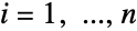 . 指定圆的数量和每个圆的半径:
n = 20;
r = BlockRandom[RandomReal[{0.5, 1.5}, n], RandomSeeding -> 234];
如果  是圆
 的圆心,则目标是最小化
 . 可将目标转换为最小化
 和
 :
objectiveConstraint = Table[-s <= Norm[c[i], Infinity] + r[[i]] <= s, {i, n}];nonOverlapConstraint = Table[Norm[c[i] - c[j]] >= r[[i]] + r[[j]],
{i, 1, n}, {j, i + 1, n}];vars = Append[Table[Element[c[i], Vectors[2, Reals]], {i, n}], Element[s, Reals]];
Short[res = NMinimize[{s, objectiveConstraint, nonOverlapConstraint}, vars, Method -> "DifferenceOfConvex"], 5]
Graphics[{Table[Circle[c[i], r[[i]]], {i, n}], {FaceForm[None], EdgeForm[StandardGray], Rectangle[{-s, -s}, {s, s}]}}] /. res[[2]]Sum[Area[Disk[c[i], r[[i]]]], {i, n}] / Area[Rectangle[{-s, -s}, {s, s}]] /. res[[2]]数据拟合问题 (3)

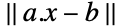
{a, b} = IconizedObject[«Block»];NMinimize[{Norm[Inactive[Plus][a.x, -b]], x1}, x]将三次曲线拟合到离散数据,使数据的第一个和最后一个点位于曲线上:
data = IconizedObject[«Block»];用 DesignMatrix 构建矩阵:
a = DesignMatrix[data, {1, x, x^2, x^3}, x];
b = data[[All, 2]];pointConstraints = {a[[1]].λ == b[[1]], a[[-1]].λ == b[[-1]]};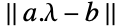

res = NMinimize[{Norm[Inactive[Plus][a.λ, -b]], pointConstraints}, λ]Show[Plot[Evaluate[{1, x, x^2, x^3}.λ /. res[[2]]], {x, 0, 1}, Epilog -> {Red, PointSize[0.03], Point[data[[{1, -1}]]]}], ListPlot[data]]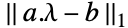
data = IconizedObject[«Block»];

bases = Sqrt[1 + (x - #) ^ 2]& /@ Subdivide[-3, 3, 10];
input = DesignMatrix[data, bases, x, IncludeConstantBasis -> False];
output = data[[All, 2]];res = NMinimize[{Norm[Inactive[Plus][a.λ, -b], 1], a == input, b == output}, λ]Plot[Evaluate[bases.λ /. res[[2]]], {x, -3, 3}, Epilog -> {PointSize[0.008], Point[data]}]Plot[{Sin[2x] + Cos[x ^ 2], Evaluate[bases.λ /. res[[2]]]}, {x, -3, 3}, PlotLegends -> {"Reference", "SubscriptBox[L, 1]fit"}]分类问题 (5)



{set1, set2} = IconizedObject[«Block»];对于此分隔问题,第 1 组点必须满足 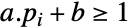 ,第 2 组点必须满足
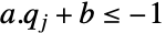 :
constraints = {set1.a + b1, set2.a + b-1};
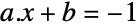
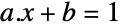
res = NMinimize[{Norm[a], constraints}, {a, b}]line = a.{x, y} + b /. res[[2]]Show[RegionPlot[line ≤ 0, {x, 0, 1}, {y, 0, 1}], ListPlot[{set1, set2}, PlotMarkers -> {Automatic, PointSize[0.025]}]]

{set1, set2} = IconizedObject[«Block»];
dataplot = ListPointPlot3D[{set1, set2}, Sequence[...]]
用 DesignMatrix 构建两组点的二次多项式数据矩阵:
{data1, data2} = DesignMatrix[#, {x, x^2, y, y^2, x y}, {x, y}]& /@ {set1, set2};对于此分隔问题,第 1 组必须满足 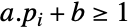 ,第 2 组必须满足
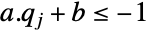 :
constraints = {data1.a + b1, data2.a + b-1};
res = NMinimize[{Norm[a], constraints}, {a, b}, PrecisionGoal -> 3]poly = (a.{1, x, x^2, y, y^2, x y} + b) /. res[[2]]Show[dataplot, ContourPlot3D[poly == 0, {x, -1.5, 1.5}, {y, -1.5, 1.5}, {z, -1, 1}, Sequence[...]]]将给定的点集  分成不同的组. 可通过最小化
 找出每组的中心
 来完成,其中
 是给定的局部核,
 是给定的惩罚参数:
x = IconizedObject[«Block»];
{n, dim} = Dimensions[x];
centers = Indexed[μ, #]& /@ Range[n];
核  为使得
 ,否则
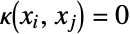 成立的
 -近邻 (
 ) 函数. 对于此问题,选择
 :
kNN = Nearest[x -> Automatic][x, 10];
κ = SparseArray[Join@@Table[Thread[{i, kNN[[i]]}], {i, n}] -> 1, {n, n}];
c1 = Table[Norm[Inactive[Plus][Indexed[x, {i}], -Indexed[μ, {i}]]], {i, n}];
c2 = Flatten[Table[κ[[i, j]]Norm[Indexed[μ, {i}] - Indexed[μ, {j}], 1], {i, 1, n}, {j, i + 1, n}]];
objective = Total[c1 ^ 2] / 2 + 10 Total[c2];vars = Table[Indexed[μ, {i}]∈Vectors[dim, Reals], {i, n}];res = NMinimize[objective, vars];对于每个数据点,都有一个对应的中心. 属于同一个组的数据将有相同的中心值:
allCenters = centers /. res[[2]];
cvals = Map[First, Gather[allCenters, Norm[#1 - #2] ≤ 0.001&]]gpts = Table[Pick[x, Map[Norm[# - ci] ≤ 0.001&, allCenters]], {ci, cvals}];
Show[ListPlot[gpts, PlotStyle -> PointSize[0.02]], ListPlot[allCenters, PlotStyle -> {PointSize[0.03], Magenta}]]给定一组正整数,将这些整数划分为两个不重叠的子集,使得两个子集的和之间的差最小. 定义列表:
n = 10;
list = BlockRandom[RandomInteger[{1, 1000}, n], RandomSeeding -> 123]
定义一个接受值 –1 或 1 的二进制变量. 如果列表中的某个元素属于子集 1,则与其关联的二进制变量的值为 –1. 对于子集 2,关联的二进制变量为 1:
vars = Table[x[i], {i, n}];
binaryConstraints = Table[{Abs[x[i]] == 1, x[i]∈Integers}, {i, 1, n}];objective = Abs[list . vars];NMinimize[objective, binaryConstraints, vars]给定一组不同重量的物体和两个袋子,找到可以放入两个袋子且不超过袋子的承重能力的总重量最大的物体. 定义物体的数量和重量:
nObjects = 20;
weights = BlockRandom[RandomInteger[{1, 1000}, nObjects], RandomSeeding -> 123]
用二进制变量来决定一个物体应被放入第一个袋子还是第二个袋子,或者不放入:
binaryConstraints = {0a1, 0b1, 0a + b1};weightConstraints = {0 <= weights.a <= 5000, 0 <= weights.b <= 5000};objective = -(weights.(a + b));sol = NMinimize[objective, {binaryConstraints, weightConstraints}, {a∈Vectors[nObjects, Integers], b∈Vectors[nObjects, Integers]}]二进制变量  与放入第一个袋子的物体相关联. 变量
 是
 的补集. 袋子的重量是:
Map[weights.# /. sol[[2]]&, {a, b}]图像处理 (1)
image = ImageResize[ColorConvert[ExampleData[{"TestImage", "House"}], "Grayscale"], 75]data = ImageData[image];
SeedRandom[123];
mask = RandomChoice[{0.4, 0.6} -> {0, 1}, Dimensions[data]];
corruptedData = mask * data;
Image[corruptedData]

{n, m} = Dimensions[data];objective = Total[Flatten[Table[Norm[{Indexed[u, {i + 1, j}] - Indexed[u, {i, j}], Indexed[u, {i, j + 1}] - Indexed[u, {i, j}]}], {i, n - 1}, {j, m - 1}]]];

knownPos = SparseArray[mask]["NonzeroPositions"];constraint = Map[Indexed[u, #] == data[[Sequence@@#]]&, knownPos];sol = NMinimize[{objective, constraint}, u∈Matrices[{n, m}, Reals]];Image[u /. sol[[2]]]设施选址问题 (1)


clientPos = {{0, 0}, {1, 0}, {3 / 2, 1}, {-1 / 2, 1}, {1 / 2, 3 / 2}, {1 / 2, 1 / 2}, {0, 3 / 2}, {1, 1}, {0, 1}, {3 / 2, 3 / 2}};
nTowers = 3;
nClients = Length[clientPos];
每个基站消耗的功率与其范围成正比,由  给出. 目的是最大程度地降低功耗:
objective = Sum[Erf[r[i] ^ 1.5], {i, nTowers}];


decisionConstraint = 0z1;m = 20;
distConstraint = Table[Norm[{p[j, 1], p[j, 2]} - clientPos[[i]]] -
m * (1 - Indexed[z, {i, j}]) ≤ r[j], {i, nClients}, {j, nTowers}];coverageConstraint = Total[z, {2}]1;maxCoverageConstraint = Table[0 ≤ r[j] ≤ 1, {j, nTowers}];vars = Flatten[{Table[{p[j, 1], p[j, 2], r[j]}, {j, nTowers}], z∈Matrices[{nClients, nTowers}, Integers]}];Quiet[res = NMinimize[{objective, decisionConstraint,
distConstraint, coverageConstraint, maxCoverageConstraint}, vars]]towerPos = Table[{p[i, 1], p[i, 2]}, {i, nTowers}] /. res[[2]];
towerRange = Table[r[i], {i, nTowers}] /. res[[2]];Graphics[{{Orange, PointSize[0.04], Point[towerPos]}, {Green, PointSize[0.02], Point[clientPos]}, {...}}, Frame -> True]投资组合优化 (1)
求如何在六只股票之间分配资本  ,在最大程度地降低风险的同时最大化回报:
{μ, Σ} = Block[...];

return = μ.w;

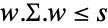
risk = w.Σ.w;
riskConstraint = risk ≤ s;
目标是最大化收益,同时在指定的风险规避参数的情况下最大程度地降低风险:
objective[α_ ? NumericQ] := -(return - α s);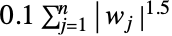
marketConstraints = Table[Abs[Indexed[w, i]] ^ 1.5 ≤ Indexed[t, i], {i, 6}];
weightConstraints = {w0, Total[w] + 0.1Total[t] == 1};frontier = Table[res = Quiet@NMinimize[{objective[α],
riskConstraint, weightConstraints, marketConstraints}, {w, s, t∈Vectors[6, Reals]}];
{risk, return} /. res[[2]], {α, Subdivide[0, 10, 100]}];

randomRiskReturns = Table[{risk, return}, {w, Table[...]}];
Show[ListPlot[frontier, ...], ListPlot[randomRiskReturns, Rule[...]]]riskAversionParameter = N@{1 / 1000, 1 / 100, 1 / 2, 1, 5, 10, 15, 20};
res = Table[{α, return, Quiet@Append[w, 1 - Total[w]]} /.
Quiet@NMinimize[{objective[α],
riskConstraint, weightConstraints, marketConstraints}, {w, s, t∈Vectors[6, Reals]}][[2]], {α, riskAversionParameter}];通过考虑市场成本,可以获得低风险规避参数的多样化投资组合,但是当风险规避参数较高时,由于购买的是分散程度较低的股票,市场影响成本占主导地位:
Legended[BarChart[res[[All, -1]], ...], SwatchLegend[...]]轨迹优化 (1)
找到一条可以绕过圆形障碍物并使得从起点到终点距离最小化的路径:
p = {{2, 2}, {7, 6}, {3, 5}, {4, 8}, {8, 9}, {6, 2.5}};
r = {1, 1.3, 1.5, 1, 0.7, 1.5};
{start, end} = {{0, 0}, {10, 10}};
domain = Graphics[{MapThread[Circle[#1, #2]&, {p, r}],
	{PointSize[0.02], Point[{start, end}]}}, Frame -> True]
路径可分解为  个不同的点. 这些点之间的距离必须小于
 ,其中
 是要最小化的长度:
n = 30;
distanceConstraints = Table[Inactive[Norm][x[i] - x[i - 1]] <= l / n, {i, n}];objectConstraints = Table[Inactive[Norm][-p[[j]] + x[i]] >= r[[j]], {i, 1, n}, {j, 1, 6}];positionConstraints = {x[0] == start, x[n] == end};vars = Append[Table[x[i]∈Vectors[2, Reals], {i, 0, n}], l∈Reals];
Short[res = NMinimize[{l, distanceConstraints,
objectConstraints, positionConstraints}, vars, Method -> "DifferenceOfConvex"], 2]pts = vars[[1 ;; -2, 1]] /. res[[2]];
Show[domain, Graphics[{Red, Point[pts]}]]制造业问题 (3)
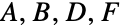



teethConstraints = {12gearTeeth60, gearTeeth∈Vectors[4, Integers]};
gearRatio = (Indexed[gearTeeth, 2]Indexed[gearTeeth, 3]) / (Indexed[gearTeeth, 1]Indexed[gearTeeth, 4]);
NMinimize[Abs[(1 / 6.931) - gearRatio], teethConstraints, gearTeeth]最大限度地降低压力容器的制造成本. 该容器是一个长度为  、半径为
 的圆柱壳,管的两端各有一个半球盖:
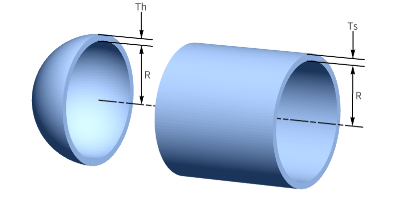
volumeConstraint = π R^2L + (4 / 3)π R^3 >= 1296000;壳的厚度为  ,半球盖的厚度为
 . 壳和半球盖的厚度有指定的上限和下限,且必须大于半径的一定比例:
thicknessConstraints = {1.1 <= Subscript[T, s] <= 2, 0.6 <= Subscript[T, h] <= 2, Subscript[T, s] >= Subscript[c, 1] R, Subscript[T, h] >= Subscript[c, 2]R};thicknessIntegerConstraints = {Subscript[T, s] == Subscript[c, k]Subscript[k, 1], Subscript[T, h] == Subscript[c, k]Subscript[k, 2], Subscript[k, 1] >= 1, Subscript[k, 2] >= 1,
Subscript[k, 1]∈Integers, Subscript[k, 2]∈Integers};dimensionConstraints = {0 <= R <= 100, 0 <= L <= 240};
materialCosts = 2π ρ (Subscript[c, s] Subscript[T, s] R L + Subscript[c, h] R^2 Subscript[T, h]);shellWeldCost = Subscript[c, w]π ρ(Subscript[T, s] / Cos[π / 6])^2(60 / 360)(2 L);
headWeldCost = Subscript[c, w]π ρ(Subscript[T, s] / Cos[π / 6])^2(60 / 360)(4π R);totalCost = shellWeldCost + headWeldCost + materialCosts;constants = {Subscript[c, 1] -> 0.0193, Subscript[c, 2] -> 0.00954, Subscript[c, s] -> 0.35, Subscript[c, h] -> 1, Subscript[c, w] -> 8, Subscript[c, k] -> 0.0625, ρ -> 0.283}NMinimize[{totalCost, volumeConstraint,
thicknessConstraints, thicknessIntegerConstraints, dimensionConstraints} /. constants, {R, L, Subscript[T, s], Subscript[T, h], Subscript[k, 1], Subscript[k, 2]}]设计一个最小体积螺旋压缩弹簧,卷绕直径为  ,弹簧线的直径为
 ,受轴向载荷限制的弹簧圈数为
 :
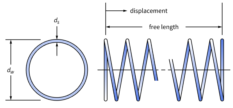
springVolume = π Subscript[d, w]Subscript[d, s]^2(Subscript[n, coils] + 2) / 4;弹簧上的剪切应力取决于允许的最大轴向载荷  ,并且必须低于最大允许应力
 :
k = With[{c = (Subscript[d, w] / Subscript[d, s])}, (4c - 1) / (4c - 4) + (0.615) / c];
shearStressConstraint = 8k Subscript[P, max]Subscript[d, w] / (π Subscript[d, s]^3) <= Subscript[S, max];δ = (8Subscript[P, max]Subscript[d, w]^3Subscript[n, coils]) / (11500000 Subscript[d, s]^4);
springLengthConstraint = (δ + 1.05(Subscript[n, coils] + 2)Subscript[d, s]) <= Subscript[l, max];springWireDiameterConstraint = Subscript[d, s] >= Subscript[d, sMin];
springWindingDiameterConstraint = Subscript[d, w] + Subscript[d, s] <= Subscript[d, max];

springDiameterRatioConstraint = Subscript[d, w] >= 3Subscript[d, s];

deflectionConstraint = Subscript[δ, min] <= δ <= Subscript[δ, max];

loadDeflectionConstraint = Subscript[P, load] + k Subscript[δ, w] <= Subscript[P, max];螺旋弹簧由音乐钢丝弹簧钢 ASTM A228 制成,钢丝直径必须从一组预定直径中选择:
wireDiameters = {0.009, 0.0095, 0.0104, 0.0118, 0.0128, 0.0132, 0.014, 0.015, 0.0162, 0.0173, 0.018, 0.020, 0.023, 0.025, 0.028, 0.032, 0.035, 0.041, 0.047, 0.054, 0.063, 0.072, 0.080, 0.092, 0.105, 0.120, 0.135, 0.148, 0.162, 0.177, 0.192, 0.207, 0.225, 0.244, 0.263, 0.283, 0.307, 0.331, 0.362, 0.394, 0.4375, 0.5};
binaryConstraints = {wireDiameters.b == Subscript[d, s], Total[b] == 1, 0b1, b∈Vectors[Length[wireDiameters], Integers]};constants = {Subscript[P, load] -> 300, Subscript[P, max] -> 1000, Subscript[S, max] -> 189000, Subscript[δ, w] -> 1.25, Subscript[δ, min] -> 1.78, Subscript[δ, max] -> 6, Subscript[l, max] -> 14, Subscript[d, max] -> 3, Subscript[d, sMin] -> 0.2};allConstraints = {shearStressConstraint, springLengthConstraint, springWireDiameterConstraint, springWindingDiameterConstraint, springDiameterRatioConstraint, deflectionConstraint, loadDeflectionConstraint, binaryConstraints, 0 <= Subscript[n, coils] <= 100} /. constants;NMinimize[springVolume, allConstraints, {Subscript[d, s], Subscript[d, w], Subscript[n, coils]∈Integers, b}]属性和关系 (9)
NMinimize 给出最小值,并以规则形式给出使结果最小化的变量值:
NMinimize[{x.x + y, Norm[x + y] ≤ 1}, {Element[x, Vectors[2, Reals]], y}]NArgMin 给出使结果最小化的值的列表:
NArgMin[{x.x + y, Norm[x + y] ≤ 1}, {Element[x, Vectors[2, Reals]], y}]NMinValue 只给出最小值:
NMinValue[{x.x + y, Norm[x + y] ≤ 1}, {Element[x, Vectors[2, Reals]], y}]NMinimize[{x ^ 2 + y ^ 2, x + 2 y ≥ 3}, {x, y}]NMaximize[{-(x ^ 2 + y ^ 2), x + 2 y ≥ 3}, {x, y}]对于凸问题,可用 ConvexOptimization 获取解的其他属性:
NMinimize[{x ^ 2 + y ^ 2, x + 2 y ≥ 3}, {x, y}]ConvexOptimization[x ^ 2 + y ^ 2, x + 2 y ≥ 3, {x, y}, {"PrimalMinimumValue", "PrimalMinimizerRules"}]ConvexOptimization[x ^ 2 + y ^ 2, x + 2 y ≥ 3, {x, y}, "DualMaximizer"]对于含有参数的凸问题,用 ParametricConvexOptimization 给出 ParametricFunction:
pfun = ParametricConvexOptimization[x + 2 y, (x - α) ^ 2 + (y - β) ^ 2 ≤ 1, {x, y}, {α, β}, {"PrimalMinimumValue", "PrimalMinimizerRules"}]可通过计算 ParametricFunction 求得参数的值:
{pfun[0., 0.], pfun[.5, 1.], pfun[2., 1.]}用 NMinimize 定义参数化问题的函数:
fun[α_ ? NumericQ, β_ ? NumericQ]  := NMinimize[{x + 2 y, (x - α) ^ 2 + (y - β) ^ 2 ≤ 1}, {x, y}];
{fun[0., 0.], fun[.5, 1.], fun[2., 1.]}testData = RandomReal[{0, 4}, {1000, 2}];
{First[AbsoluteTiming[pfun @@@testData]], First[AbsoluteTiming[fun @@@ testData]]}也可以计算 ParametricFunction 的导数:
D[pfun[α, β], {{α, β}}] /. {α -> 2., β -> 1.}对于含有参数化约束条件的凸问题,RobustConvexOptimization 将找到适用于所有可能参数值的最优值:
{rMinValue, rMin} = RobustConvexOptimization[2x + 3y, x + y ≥ α && x - y ≤ β && -1 ≤ α ≤ 1 && 0 ≤ β ≤ 1, {x, y}, {α, β}, {"PrimalMinimumValue", "PrimalMinimizerRules"}]对于特定参数值,NMinimize 可能会找到更小的值:
NMinimize[{2x + 3y, x + y ≥ α && x - y ≤ β && α == 0 && β == 0}, {x, y}](x + y ≥ α && x - y ≤ β /. Last[%]) /. {α -> 1, β -> 1}fun[α_, β_] /; (-1 ≤ α ≤ 1 && 0 ≤ β ≤ 1) :=
NMinValue[{2x + 3y, x + y ≥ α && x - y ≤ β}, {x, y}];testValues = RandomVariate[UniformDistribution[{{-1, 1}, {0, 1}}], 100];
AllTrue[testValues, ((fun@@#) ≤ rMinValue)&]FindMinimum 试图找到一个局部最小值,NMinimize 的目的在于找到全局最小值:
objective = -100 / ((x - 1)^2 + (y - 1)^2 + 1) - 200 / ((x + 1)^2 + (y + 2)^2 + 1);
NMinimize[{objective, x^2 + y^2 > 3 }, {x, y}]FindMinimum[{objective, x^2 + y^2 > 3 }, {{x, 2}, y}]ContourPlot[objective, {x, -3, 2}, {y, -3, 2}, ...]FindFit 可以用 NMinimize 来求全局最佳拟合,下面先设立一个模型:
model = a + bCos[2Pict] + dSin[2Piet];
parameters = {a, b, c, d, e};f[t_] := Evaluate[model /. {a -> 0.2, b -> 0.3, c -> 0.1, d -> 0.9, e -> 0.55}];
data = {#, f[#]}& /@ Table[t, {t, 0, 2Pi, .1}];默认情况下,FindFit 只求出局部最佳拟合:
ffsol = FindFit[data, model, parameters, t];
lp = ListPlot[data, PlotStyle -> {PointSize[0.02]}, DisplayFunction -> Identity];nfp = Plot[model /. ffsol, {t, 0, 2Pi}, DisplayFunction -> Identity];
Show[lp, nfp, DisplayFunction -> $DisplayFunction]
用 NMinimize 方法求全局最佳拟合:
ffsol = FindFit[data, model, parameters, t, Method -> NMinimize];
nfp = Plot[model /. ffsol, {t, 0, 2Pi}, DisplayFunction -> Identity];
Show[lp, nfp, DisplayFunction -> $DisplayFunction]
用 RegionDistance 和 RegionNearest 计算距离和最近的点:
ℛ = Cone[{{-1, 0, 1}, {2, 3, 4}}, 3];
p = {3., 2., 1.};RegionDistance[ℛ, p]RegionNearest[ℛ, p]这两者都可以使用 NMinimize 计算:
NMinimize[Norm[{x, y, z} - p], {x, y, z}∈ℛ]Graphics3D[{ℛ, {PointSize[Large], {Green, Point[p]}, {Red, Point[{x, y, z} /. %[[2]]]}}}]用 RegionBounds 计算边界框:
f = x^4 + 3. x^2 y + 2. x^2 y^2 - y^3 + y^4 ≤ 0;
ℛ = ImplicitRegion@@{f, {x, y}}RegionBounds[ℛ]用 NMaximize 和 NMinimize 做同样的计算:
{{x1, x2}, {y1, y2}} = {NMinimize[#, {x, y}∈ℛ][[1]], NMaximize[#, {x, y}∈ℛ][[1]]}& /@ {x, y}Show[{Graphics[{LightBlue, Rectangle[{x1, y1}, {x2, y2}]}], RegionPlot[f, {x, x1 - 1, x2 + 1}, {y, y1 - 1, y2 + 1}]}]可能存在的问题 (3)
对于非线性函数,NMinimize 的某些方法有时可能只能找到局部最小值:
sol = NMinimize[-x Sin[x] + 3 Cos[x] + x / 1000, x, Method -> "NelderMead"]Plot[-x Sin[x] + 3 Cos[x] + x / 1000, {x, -20, 20}, Epilog -> {Red, PointSize[0.04], Point[{x /. sol[[2]], sol[[1]]}]}]NMinimize[-x Sin[x] + 3 Cos[x] + x / 1000, {x, -20, 20}, Method -> "NelderMead"]NMinimize[-x Sin[x] + 3 Cos[x] + x / 1000, x]对于某些方法,NMinimize 找到的是圆盘上二维函数的局部最小值:
NMinimize[{Cos[x] - Exp[(x - 0.5) y], x ^ 2 + y ^ 2 < 1}, {x, y}, Method -> "NelderMead"]NMinimize[{Cos[x] - Exp[(x - 0.5) y], x ^ 2 + y ^ 2 < 1}, {{x, -1, 0}, y}, Method -> "NelderMead"]ContourPlot[Cos[x] - Exp[(x - 0.5)y], {x, -1, 1}, {y, -1, 1}, ...]f1[a_] := NIntegrate[(x - a) ^ 2, {x, 0, 10}]f1[2]对符号参数应用函数,NIntegrate 发出一条消息:
f1[q]
当该函数与其他数值函数(如 NMinimize)一起使用时,也会导致警告消息:
NMinimize[f1[a], a]



定义一个仅在其参数为数值时才进行计算的函数,以避免出现这些消息:
f2[a_ ? NumericQ] := NIntegrate[(x - a) ^ 2, {x, 0, 10}]f2[π]f2[q]现在,该函数可与其他数值函数(如 NMinimize)一起使用:
NMinimize[f2[a], a]文本
Wolfram Research (2003),NMinimize,Wolfram 语言函数,https://reference.wolfram.com/language/ref/NMinimize.html (更新于 2024 年).
CMS
Wolfram 语言. 2003. "NMinimize." Wolfram 语言与系统参考资料中心. Wolfram Research. 最新版本 2024. https://reference.wolfram.com/language/ref/NMinimize.html.
APA
Wolfram 语言. (2003). NMinimize. Wolfram 语言与系统参考资料中心. 追溯自 https://reference.wolfram.com/language/ref/NMinimize.html 年