

TruncatedDistribution
TruncatedDistribution[{xmin,xmax},dist]
dist の値が xminから xmaxまでになるように切断することで得られる分布を表す.
TruncatedDistribution[{{xmin,xmax},{ymin,ymax},…},dist]
多変量分布 dist の値が xminから xmaxまで,yminから ymaxまでという具合になるように切断することで得られる分布を表す.
詳細
- TruncatedDistribution[{xmin,xmax},dist]の確率密度は,
 については
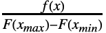 で与えられ(
 は dist の確率密度関数,
 は dist の累積分布関数),その他の場合は0である.
- {xmin,xmax}の一般的なケース
-
{-∞,xmax} 上から切断 {xmin,∞} 下から切断 {xmin,xmax} 二重に切断 {-∞,∞},None 切断なし - TruncatedDistributionは,Mean,CDF,RandomVariate等の関数とともに使うことができる.
予備知識
- TruncatedDistribution[{xmin,xmax},dist]は,区間
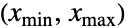 におけるすべての
 について定数倍し,
 については常に0になるデータをモデル化する統計分布を表す.非切断,以下を切断,以上を切断,二重切断という語は,{xmin,xmax}がそれぞれ{-∞,∞},{xmin,∞},{-∞,xmax},{xmin,xmax},の形であるものを説明するのに対し,一変量 dist は連続分布(NormalDistribution,GammaDistributionまたはBetaDistribution)あるいは離散分布(PoissonDistribution,BinomialDistributionまたはBernoulliDistribution)のいずれかであり,変換,打ち切りあるいは切断(それぞれTransformedDistribution,CensoredDistribution,TruncatedDistribution)あるいは既知の分布によって定義することができる.
- 多変量のTruncatedDistribution[{{
 ,
 },… ,{
 ,
 }},dist]は,一変量分布との類似に基づいて定義され,したがって,多変量分布 dist から取られ,
 番目の成分
 が区間
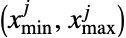 内に収まるように切断されたベクトル
 の分布を表す.一変量の場合と同じように,多変量分布 dist も連続分布(例:MultinormalDistribution)あるいは離散分布(例:MultivariateHypergeometricDistribution)であり,(それぞCopulaDistributionおよびProductDistributionを使って)既知の分布のコピュラ分布あるいは積分布として定義することができる.
- 切断分布は,データ集合が「条件を満たす」とみなされる範囲の外側の値を含む場合に使われる.例えば,納税者の集合中の最初の
 人を監査する場合(
 ),監査対象となった人について行われる統計分析の結果は,監査対象とはならなかった
 人の納税者についての情報が保存されていない切断データとなる.このようなデータは,生存分析,金融,保険数理,経済等の分野では一般的であり,そのようなデータの分析用のさまざまな特化された統計ツール(例:切断回帰)が存在する.
- TruncatedDistributionはCensoredDistributionと混同されることがよくあるが,切断分布が切断区間上の確率を分布させるのに対し打ち切り分布は打ち切り区間の最後に完全な確率を置く点でこの2つは根本的に異なる.CensoredDistribution[{xmin,xmax},dist]は,定義上,TransformedDistribution[g,xdist]に等しい.ただし,g は
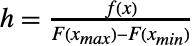 についてPiecewise[{{0,x<=xmin},{h,xmin<x<xmax},{0,x>=xmax}}]によって与えられる.
 は dist の累積密度関数であり,
 はその累積分布関数である.
例題
すべて開く すべて閉じる例 (3)
TruncatedDistribution[{0, ∞}, NormalDistribution[]]TruncatedDistribution[{a, b}, DiscreteUniformDistribution[{a, b}]]𝒟 = TruncatedDistribution[{-∞, 0.5}, 𝒹 = CauchyDistribution[0, 1]];Plot[{Legended[PDF[𝒹, x], "𝒹"], Legended[PDF[𝒟, x], "𝒟"]}, {x, -2, 2}, Filling -> Axis]𝒫 = MultivariatePoissonDistribution[10, {3, 9}];
𝒟 = TruncatedDistribution[{{5, 15}, {12, 25}}, 𝒫];{DiscretePlot3D[PDF[𝒟, {x, y}]//Evaluate, {x, 1, 20}, {y, 5, 30}, PlotRange -> {0, 0.02}, ExtentSize -> Full, PlotLabel -> "𝒟"], DiscretePlot3D[PDF[𝒫, {x, y}]//Evaluate, {x, 1, 20}, {y, 5, 30}, PlotRange -> {0, 0.02}, ExtentSize -> Full, PlotLabel -> "𝒫"]}スコープ (35)
基本的な用法 (9)
LeftTruncated𝒟 = TruncatedDistribution[{-1, ∞}, NormalDistribution[]];
RightTruncated𝒟 = TruncatedDistribution[{-∞, 1}, NormalDistribution[]];
DoubleTruncated𝒟 = TruncatedDistribution[{-1, 1}, NormalDistribution[]];Table[Plot[{PDF[m, x], PDF[NormalDistribution[], x]}, {x, -3, 3}, Filling -> Axis, Exclusions -> None], {m, {LeftTruncated𝒟, RightTruncated𝒟, DoubleTruncated𝒟}}]Table[Plot[{CDF[m, x], CDF[NormalDistribution[], x]}, {x, -3, 3}, Filling -> Axis, Exclusions -> None], {m, {LeftTruncated𝒟, RightTruncated𝒟, DoubleTruncated𝒟}}]LeftTruncated𝒟 = TruncatedDistribution[{4, ∞}, PoissonDistribution[7]];
RightTruncated𝒟 = TruncatedDistribution[{-∞, 9}, PoissonDistribution[7]];
DoubleTruncated𝒟 = TruncatedDistribution[{4, 9}, PoissonDistribution[7]];Table[DiscretePlot[{PDF[m, x], PDF[PoissonDistribution[7], x]}, {x, 0, 12}, ExtentSize -> 0.5], {m, {LeftTruncated𝒟, RightTruncated𝒟, DoubleTruncated𝒟}}]PDF[LeftTruncated𝒟, 4]PDF[RightTruncated𝒟, 9]//N{PDF[DoubleTruncated𝒟, 4], PDF[DoubleTruncated𝒟, 9]}//N𝒟 = TruncatedDistribution[{-∞, 1 / 2}, 𝒹 = StudentTDistribution[3]];Plot[{Legended[PDF[𝒹, x], "𝒹"], Legended[PDF[𝒟, x], "𝒟"]}, {x, -3, 3}, Filling -> Axis, Exclusions -> None]PDF[𝒟, x]𝒟 = TruncatedDistribution[{3, ∞}, 𝒹 = BinomialDistribution[10, 1 / 4]];DiscretePlot[{Legended[PDF[𝒹, x], "𝒹"], Legended[PDF[𝒟, x], "𝒟"]}, {x, 0, 8}, ExtentSize -> 1 / 2]{Mean[𝒹], Mean[𝒟]}//N{StandardDeviation[𝒹], StandardDeviation[𝒟]}//N𝒟 = TruncatedDistribution[{-3, 7}, 𝒹 = CauchyDistribution[0, 1]];{Mean[𝒟], Mean[𝒹]}{Variance[𝒟], Variance[𝒹]}//N𝒟 = TruncatedDistribution[{{1 / 4, 1 / 2}, {1 / 5, 4 / 5}}, 𝒹 = DirichletDistribution[{1, 3, 2}]];Plot3D[{Legended[PDF[𝒟, {x, y}], "𝒟"], Legended[PDF[𝒹, {x, y}], "𝒹"]}//Evaluate, {x, 0, 1}, {y, 0, 1}, PlotRange -> All, PlotPoints -> 35, AxesLabel -> Automatic ]NExpectation[x ^ 2 + y, {x, y}𝒟]Table[Moment[𝒟, r], {r, {{1, 2}, {2, 3}, {2, 2}}}]//N𝒟 = TruncatedDistribution[{{2, 10}, {4, 12}, {3, 19}}, 𝒹 = MultinomialDistribution[20, {1 / 3, 1 / 2, 1 / 6}]];Probability[{x, y, z} == {11, 2, 7}, {x, y, z}#]& /@ {𝒟, 𝒹}data = RandomVariate[𝒟, 10 ^ 4];{Mean[data], Mean[𝒟]//N}𝒟 = TruncatedDistribution[{{0, 14}, {0, 10}}, 𝒹 = NegativeMultinomialDistribution[20, {0.3, 0.2}]];{DiscretePlot3D[PDF[𝒟, {x, y}]//Evaluate, {x, 0, 20}, {y, 0, 20}, ExtentSize -> Full, PlotRange -> {0, 0.02}], DiscretePlot3D[PDF[𝒹, {x, y}]//Evaluate, {x, 0, 20}, {y, 0, 20}, ExtentSize -> Full, PlotRange -> {0, 0.02}]}{Skewness[𝒟], Skewness[𝒹]}//Column{Kurtosis[𝒟], Kurtosis[𝒹]}//ColumnEstimatedDistributionを使って切断区間を推定する:
𝒟 = TruncatedDistribution[{-1, 0}, NormalDistribution[]];
sample = RandomVariate[𝒟, 10 ^ 2];edist = EstimatedDistribution[sample, TruncatedDistribution[{a, b}, NormalDistribution[]]]パラメトリック分布 (7)
𝒟 = TruncatedDistribution[{1, ∞}, 𝒹 = ExponentialDistribution[1 / 3]];Plot[{Legended[PDF[𝒹, x], "𝒹"], Legended[PDF[𝒟, x], "𝒟"]}, {x, 0, 5}, Filling -> Axis]CDF[𝒟, x]{Mean[𝒟], Variance[𝒟], Skewness[𝒟], Kurtosis[𝒟]}{Mean[𝒹], Variance[𝒹], Skewness[𝒹], Kurtosis[𝒹]}𝒟 = TruncatedDistribution[{-∞, 3}, 𝒹 = ZipfDistribution[10, 1 / 3]];DiscretePlot[{Legended[PDF[𝒹, x], "𝒹"], Legended[PDF[𝒟, x], "𝒟"]}//Evaluate, {x, 0, 10}, ExtentSize -> 1 / 2]PDF[𝒟, x]PDF[ZipfDistribution[3, 1 / 3], x]UniformDistributionの切断分布を定義する:
𝒟 = TruncatedDistribution[{0, 4}, UniformDistribution[{-2, 6}]];PDF[𝒟, x]PDF[UniformDistribution[{0, 4}], x]DiscreteUniformDistributionの切断分布を定義する:
𝒟 = TruncatedDistribution[{0, 4}, DiscreteUniformDistribution[{-2, 6}]];PDF[𝒟, x]PDF[DiscreteUniformDistribution[{0, 4}], x]切断は左端点を含まず,よって結果の離散分布は以下の様になる:
PDF[DiscreteUniformDistribution[{1, 4}], x]𝒟 = TruncatedDistribution[{{-∞, 1 / 2}, {-∞, ∞}}, 𝒹 = BinormalDistribution[1 / 7]];二変量正規分布とその切断バージョンの確率密度関数を比較する:
Plot3D[{PDF[𝒟, {x, y}], PDF[𝒹, {x, y}]}//Evaluate, {x, -3, 3}, {y, -3, 3}, PlotRange -> All, PlotPoints -> 35, PlotLegends -> {"𝒟", "𝒹"}]PDF[𝒟, {x, y}]CharacteristicFunction[𝒟, {s, t}]𝒟 = TruncatedDistribution[{{3, 12}, {4, 7}, {0, 4}}, MultinomialDistribution[13, {1 / 7, 4 / 7, 2 / 7}]];Mean[𝒟]Variance[𝒟]Skewness[𝒟]Kurtosis[𝒟]𝒟 = TruncatedDistribution[{1 / 2, 10}, 𝒹 = SuzukiDistribution[2, 1 / 2]];sample = RandomVariate[𝒟, 10 ^ 5];Show[Histogram[sample, {0, 15.5, .5}, "PDF"], Plot[{Legended[PDF[𝒹, x], "𝒹"], Legended[PDF[𝒟, x], "𝒟"]}, {x, 0, 15}, Filling -> {1 -> Axis}]]ノンパラメトリック分布 (3)
SmoothKernelDistributionを切断する:
data = RandomVariate[NormalDistribution[], 10 ^ 2];
skd = SmoothKernelDistribution[data];
𝒟 = TruncatedDistribution[{0, ∞}, skd];Plot[{Legended[PDF[skd, x], "skd"], Legended[PDF[𝒟, x], "𝒟"]}, {x, -3, 3}, Filling -> Axis]切断EmpiricalDistributionを定義する:
ed = EmpiricalDistribution[RandomVariate[WeibullDistribution[2, 3], 15]];
𝒟 = TruncatedDistribution[{0, 3}, ed];Plot[{Legended[CDF[ed, x], "ed"], Legended[CDF[𝒟, x], "𝒟"]}, {x, 0, 6}, Filling -> Axis, Exclusions -> None]切断HistogramDistributionを定義する:
hd = HistogramDistribution[RandomVariate[PoissonDistribution[9], 10 ^ 3]];
𝒟 = TruncatedDistribution[{0, 10}, hd];Plot[{Legended[PDF[hd, x], "hd"], Legended[PDF[𝒟, x], "𝒟"]}, {x, 0, 15}, Filling -> Axis, Exclusions -> None]PDF[𝒟, x]//Simplify派生分布 (10)
切断TruncatedDistributionを定義する:
𝒹 = TruncatedDistribution[{-1, 1}, NormalDistribution[2, 1 / 3]];
𝒟 = TruncatedDistribution[{0, 1}, 𝒹];PDF[𝒟, x]//FullSimplifyPDF[TruncatedDistribution[{0, 1}, NormalDistribution[2, 1 / 3]], x]FullSimplify[% - %%]切断CopulaDistributionを定義する:
𝒞 = CopulaDistribution[{"AMH", 5 / 9},     {UniformDistribution[{-1, 1}], UniformDistribution[{-2, 2}]} ];
𝒟 = TruncatedDistribution[{{-1, 0}, {-2, 0}}, 𝒞];Plot3D[Evaluate[{Legended[PDF[𝒞, {x, y}], "𝒞"], Legended[PDF[𝒟, {x, y}], "𝒟"]}], {x, -1.2, 0.5}, {y, -2.5, 1.5}, PlotRange -> All, AxesLabel -> Automatic, PlotPoints -> 35, ViewPoint -> {0.5, -2, 0.7}]切断MixtureDistributionを定義する:
ℳ = MixtureDistribution[{1, 2}, {PoissonDistribution[3], PoissonDistribution[8]}];
𝒟 = TruncatedDistribution[{4, 10}, ℳ];DiscretePlot[{Legended[PDF[ℳ, x], "ℳ"], Legended[PDF[𝒟, x], "𝒟"]}, {x, 0, 14}, ExtentSize -> 1 / 2]切断OrderDistributionを定義する:
𝒪 = OrderDistribution[{PoissonDistribution[3], 10}, 10];
𝒟 = TruncatedDistribution[{5, 8}, 𝒪];DiscretePlot[{Legended[PDF[𝒪, x], "𝒪"], Legended[PDF[𝒟, x], "𝒟"]}, {x, 0, 10}, PlotMarkers -> Automatic]ポアソンサンプルの最大値が5より大きいと仮定した場合に,6より大きくなる確率を求める:
NProbability[x > 6, x𝒟]最大値が5より大きいという仮定なしで,6より大きい確率を求める:
Probability[x > 6, x𝒪]//N切断TransformedDistributionを定義する:
𝒯 = TransformedDistribution[u ^ 2, uNormalDistribution[]];
𝒟 = TruncatedDistribution[{0, 1 / 2}, 𝒯];Plot[{Legended[PDF[𝒯, x], "𝒯"], Legended[PDF[𝒟, x], "𝒟"]}, {x, 0, 1}, Filling -> Axis]
𝒫 = TransformedDistribution[u ^ 2, uTruncatedDistribution[{0, 1 / 2}, NormalDistribution[]]];Plot[{Legended[PDF[𝒫, x], "𝒫"], Legended[PDF[𝒟, x], "𝒟"]}, {x, 0, 1}, Filling -> Axis]切断ParameterMixtureDistributionを定義する:
ℳ = ParameterMixtureDistribution[BenfordDistribution[2 + b], bBinomialDistribution[8, .7]];
𝒟 = TruncatedDistribution[{2, 7}, ℳ];DiscretePlot[{PDF[ℳ, x], PDF[𝒟, x]}, {x, 0, 10}, ExtentSize -> 1 / 2, PlotLegends -> SwatchLegend[{"ℳ", "𝒟"}]]{PDF[𝒟, 3], PDF[ℳ, 1]}切断ProductDistributionを定義する:
𝒫 = ProductDistribution[ExponentialDistribution[1 / 2], NormalDistribution[-1, 1]];
𝒟 = TruncatedDistribution[{{1, 2}, {-∞, 3}}, 𝒫];Plot3D[Evaluate[{Legended[PDF[𝒫, {x, y}], "𝒫"], Legended[PDF[𝒟, {x, y}], "𝒟"]}], {x, 0.2, 2.5}, {y, -4, 4}, AxesLabel -> Automatic, PlotPoints -> 35, PlotRange -> All, ViewPoint -> {-1, 1, 1}]PDF[𝒟, {x, y}]//FullSimplifyPDF[ProductDistribution[TruncatedDistribution[{1, 2}, ExponentialDistribution[1 / 2]], TruncatedDistribution[{-∞, 3}, NormalDistribution[-1, 1]]], {x, y}]//FullSimplifyFullSimplify[% - %%]切断MarginalDistributionを定義する:
ℳ = MarginalDistribution[NegativeMultinomialDistribution[10, {.2, .4}], 2];
𝒟 = TruncatedDistribution[{3, 8}, ℳ];DiscretePlot[{Legended[PDF[ℳ, x], "ℳ"], Legended[PDF[𝒟, x], "𝒟"]}//Evaluate, {x, 1, 20}, ExtentSize -> 1 / 2]切断CensoredDistributionを定義する:
𝒟 = TruncatedDistribution[{7, 12}, 𝒹 = CensoredDistribution[{4, ∞}, PoissonDistribution[6]]];DiscretePlot[{Legended[PDF[𝒹, x], "𝒹"], Legended[PDF[𝒟, x], "𝒟"]}//Evaluate, {x, 0, 16}, ExtentSize -> 1 / 2]QuantityDistributionの切断分布を評価するとQuantityDistributionになる:
qd = QuantityDistribution[NormalDistribution[20, 3], "DegreesCelsius"];𝒟 = TruncatedDistribution[{Quantity[16, "DegreesCelsius"], Quantity[25, "DegreesCelsius"]}, qd]Mean[𝒟]//N自動簡約 (6)
連続分布 (4)
正の軸までで切断されたGumbelDistributionはGompertzMakehamDistributionに従う:
TruncatedDistribution[{0, ∞}, GumbelDistribution[α, β]]正の軸までで切断されたNormalDistributionはHalfNormalDistributionに従う:
TruncatedDistribution[{0, ∞}, NormalDistribution[0, σ]]ParetoDistributionは切断のもとで閉じている:
TruncatedDistribution[{b, ∞}, ParetoDistribution[k, α]]UniformDistributionは切断のもとで閉じている:
TruncatedDistribution[{a, b}, UniformDistribution[{min, max}]]離散分布 (2)
DiscreteUniformDistributionは切断のもとで閉じている:
TruncatedDistribution[{a, b}, DiscreteUniformDistribution[{min, max}]]ZipfDistributionは切断のもとで閉じている:
TruncatedDistribution[{0, b}, ZipfDistribution[ρ]]TruncatedDistribution[{0, b}, ZipfDistribution[n, ρ]]アプリケーション (5)
ある食料品店では一日に販売するためにある食品を1ポンドあたり  ドルで
 ポンド仕入れる,この食品の利益はポンドあたり
 である.この食品が一日に売れる量は分布
 に従う.売れ残りはその日のうちに廃棄される.一日の利益が最大になるような
 を計算する:
Profit[x_, p_, margin_, dist_] := -x p + (p + margin) Expectation[y, yTruncatedDistribution[{0, x}, dist]]30%の利益率を仮定し,需要の分布にLogNormalDistributionを使う:
𝒟 = LogNormalDistribution[5, 1 / 5];pr = Profit[x, 1, (3/10), 𝒟]Plot[pr, {x, 0, Mean[𝒟]}, PlotPoints -> 3]FindMaximum[Refine[pr, x > 0], {x, Mean[𝒟]}, AccuracyGoal -> 3]アメリカのクランベリーの直径は平均16ミリ,標準偏差1.6ミリで正規分布に従う.クランベリーを青果として販売する場合は実の直径が最低15ミリなければならない.それより小さい場合はクランベリーソースの原料として使われる.青果として売られるクランベリーの大きさの分布を求める:
cran𝒟 = NormalDistribution[Quantity[16, "Millimeters"], Quantity[1.6, "Millimeters"]];
𝒟 = TruncatedDistribution[{Quantity[15, "Millimeters"], ∞}, cran𝒟];Plot[{Legended[PDF[cran𝒟, Quantity[x, "mm"]], "cran𝒟"], Legended[PDF[𝒟, Quantity[x, "mm"]], "𝒟"]}, {x, 10, 22}, Filling -> Axis, PlotStyle -> {Automatic, Thick}, AxesLabel -> {"mm"}]Mean[𝒟]青果として売られる実の直径が少なくとも18ミリである確率を求める:
Probability[x ≥ Quantity[18, "Millimeters"] , x𝒟]切断分布を使って裾部の長い分布の表示を制御することができる.サンプルを例に考える:
sample = RandomVariate[ParetoDistribution[1, 1 / 3], 10 ^ 3];edist = EstimatedDistribution[sample, ParetoDistribution[k, α]]Show[Histogram[sample, Automatic, "PDF"], Plot[PDF[edist, x], {x, 1, 10}, PlotStyle -> Thick]]裾部が長いため,ヒストグラムの範囲を調整し,分布を切断しなければならない:
Show[Histogram[sample, {1, 7, 0.5}, "PDF"], Plot[PDF[TruncatedDistribution[{1, 7}, edist], x], {x, 1, 10}, PlotStyle -> Thick]]ExampleData[{"Statistics", "CrabMeasures"}, "LongDescription"]CrabWidth = QuantityArray[ExampleData[{"Statistics", "CrabMeasures"}][[ ;; , 7]], "mm"];データにDagumDistributionをフィットさせる:
edist = EstimatedDistribution[CrabWidth, DagumDistribution[a, b, c]]Show[Histogram[CrabWidth, 15, "PDF", AxesLabel -> Automatic], Plot[PDF[edist, Quantity[x, "mm"]], {x, 10, 56}, PlotStyle -> Thick]]MinMax[CrabWidth]edist2 = EstimatedDistribution[CrabWidth, TruncatedDistribution[{Quantity[17, "mm"], ∞}, DagumDistribution[a, b, Quantity[c, "mm"]]], {{a, 0.2}, {b, 15}, {c, 42}}]Show[Histogram[CrabWidth, 15, "PDF", AxesLabel -> Automatic], Plot[PDF[edist2, Quantity[x, "mm"]], {x, 10, 56}, PlotStyle -> Thick]]対数尤度値を比較して,切断分布を使った方フィットの方がよいかどうかを見る:
LogLikelihood[#, CrabWidth]& /@ {edist, edist2}ある会社では長さが平均0.5インチで正規分布に従う釘を製造している.製造された釘の50%は長さの違いが0.05インチ未満であるとして,標準偏差を求める:
𝒟 = TruncatedDistribution[{Quantity[0, "Inches"], ∞}, NormalDistribution[Quantity[1/2, "Inches"], Quantity[σ, "Inches"]]];標準偏差はスペックに収まる確率が50%となることを要求すると求まる:
prob[σ_] = Probability[Abs[x - Quantity[1/2, "Inches"]] < Quantity[1/20, "Inches"], x𝒟]Plot[{prob[σ], 1 / 2}, {σ, 0.05, 0.1}, AxesLabel -> {σ, None}]FindRoot[prob[σ] == Quantity[50, "Percent"], {σ, 0.08}]特性と関係 (7)
Probability[0 < x < 1, xTruncatedDistribution[{-2, 2}, NormalDistribution[]]]//FunctionExpandProbability[0 < x < 1-2 <= x <= 2, xNormalDistribution[]]切断分布の確率密度関数では,切断された区間の内部にしか非零の値がない:
𝒟 = TruncatedDistribution[{-1, 2}, 𝒩 = NormalDistribution[]];PDF[𝒟, x]Plot[{Legended[PDF[𝒟, x], "𝒟"], Legended[PDF[𝒩, x], "𝒩"]}//Evaluate, {x, -3, 3}, Filling -> Axis]基になっている分布の特性を使って切断分布の確率密度関数を構築する:
f[x_] := PDF[NormalDistribution[], x]F[x_] := CDF[NormalDistribution[], x]pdf1 = Piecewise[{{(f[x]/F[b] - F[a]), a < x ≤ b}}]pdf2 = PDF[TruncatedDistribution[{a, b}, NormalDistribution[]], x]Simplify[pdf1 == pdf2]𝒞 = CensoredDistribution[{4, 9}, 𝒫 = PoissonDistribution[7]];
𝒯 = TruncatedDistribution[{4, 9}, 𝒫];DiscretePlot[{Legended[PDF[𝒫, x], "𝒫"], Legended[PDF[𝒯, x], "𝒯"]}, {x, 0, 12}, ExtentSize -> 1 / 2]DiscretePlot[{Legended[PDF[𝒫, x], "𝒫"], Legended[PDF[𝒞, x], "𝒞"]}, {x, 0, 12}, ExtentSize -> 1 / 2]𝒞 = CensoredDistribution[{1 / 2, ∞}, 𝒩 = NormalDistribution[0, 1 / 2]];
𝒯 = TruncatedDistribution[{1 / 2, ∞}, 𝒩];Plot[{Legended[CDF[𝒩, x], "𝒩"], Legended[CDF[𝒯, x], "𝒯"]}, {x, -2, 3}, Filling -> Axis]Plot[{Legended[CDF[𝒩, x], "𝒩"], Legended[CDF[𝒞, x], "𝒞"]}, {x, -2, 3}, Filling -> Axis]GompertzMakehamDistributionは切断WeibullDistributionに関連している:
𝒟 = TransformedDistribution[Exp[u], uGompertzMakehamDistribution[α, β]];PDF[𝒟, x]PDF[TruncatedDistribution[{1, ∞}, WeibullDistribution[α, β ^ (-1 / α)]], x]//PowerExpandFullSimplify[% - %%, x ≠ 1]切断GumbelDistributionはGompertzMakehamDistributionである:
TruncatedDistribution[{0, ∞}, GumbelDistribution[α, β]]おもしろい例題 (1)
𝒟 = ProductDistribution[NormalDistribution[], LaplaceDistribution[-1 / 2, 1]];𝒯 = TruncatedDistribution[{{-∞, 1}, {-1, ∞}}, 𝒟];Plot3D[Evaluate[{PDF[𝒟, {x, y}], PDF[𝒯, {x, y}]}], {x, -2, 2}, {y, -2, 2}, PlotStyle -> Opacity[0.7], PlotRange -> All, Mesh -> None, AxesLabel -> Automatic]テキスト
Wolfram Research (2010), TruncatedDistribution, Wolfram言語関数, https://reference.wolfram.com/language/ref/TruncatedDistribution.html (2016年に更新).
CMS
Wolfram Language. 2010. "TruncatedDistribution." Wolfram Language & System Documentation Center. Wolfram Research. Last Modified 2016. https://reference.wolfram.com/language/ref/TruncatedDistribution.html.
APA
Wolfram Language. (2010). TruncatedDistribution. Wolfram Language & System Documentation Center. Retrieved from https://reference.wolfram.com/language/ref/TruncatedDistribution.html