Asymptotic[expr,xx0]
x0の近くの expr についての漸近近似を与える.
Asymptotic[expr,{x,x0,n}]
x0の近くの expr についての漸近近似を次数 n まで与える.
Asymptotic
Asymptotic[expr,xx0]
x0の近くの expr についての漸近近似を与える.
Asymptotic[expr,{x,x0,n}]
x0の近くの expr についての漸近近似を次数 n まで与える.
詳細とオプション
- Asymptoticは,主に,厳密解が求まらない問題を解くため,あるいは計算,比較,解釈等のためにより簡単な答を得るために使われる.そのような場合,漸近近似はしばしば該当する問題を簡約したり解いたりするために十分な情報を与える.
- Asymptotic[expr,x->x0]は,expr についての漸近展開における最高次の項を計算する.SeriesTermGoalを使うとより多くの項が指定できる.
- 式 expr は,任意の関数
,Integrate,LaplaceTransformあるいはInverseLaplaceTransformで指定される積分,DSolveValueで指定される微分方程式等でよい. - 展開点 x0は,任意の有限または無限の実数または複素数でよい.
- 近似次数 n は任意の正の整数またはInfinityでよい.n がInfinityに設定されていて expr が x の解析関数なら,Asymptoticは x0の周りの expr の完全なベキ級数展開を与える. »
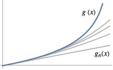
- 厳密結果が g[x]で x0における次数 n の漸近近似が gn[x]であれば,xx0のときにAsymptoticLess[g[x]-gn[x],gn[x]-gn-1[x],xx0]または g[x]-gn[x]∈o[gn[x]-gn-1[x]]である.
- 漸近近似 gn[x]はしばしば総和 gn[x]
αkϕk[x]として与えられる.{ϕ1[x],…,ϕn[x]}は xx0のときの漸近尺度 ϕ1[x]≻ϕ2[x]≻⋯>ϕn[x]である.こうすると,xx0のとき AsymptoticLess[g[x]-gn[x],ϕn[x],xx0]または g[x]-gn[x]∈o[ϕn[x]]となる. - 次は,よく含まれる漸近尺度である.
-

xx0のとき,テイラー(Taylor)スケール 

xx0のとき,ローラン(Laurent)スケール 

x±∞のとき,ローランスケール 

xx0のとき,ピュイゾー(Puiseux)スケール - 漸近近似を表すために使われる尺度は問題から自動的に推測される.多くの場合,より珍しい尺度を含めることができる.
- 次は,使用可能なオプションである.
-
AccuracyGoal Automatic 目標とする絶対確度の桁数 Assumptions $Assumptions パラメータについての仮定 GenerateConditions Automatic パラメータについての条件を含む答を生成するかどうか GeneratedParameters None 生成されたパラメータにどのように命名するか Method Automatic 使用するメソッド PerformanceGoal $PerformanceGoal パフォーマンスのどの面について最適化するか PrecisionGoal Automatic 目標精度の桁数 SeriesTermGoal Automatic 近似における項数 WorkingPrecision Automatic 内部計算の精度 - GenerateConditionsにデフォルト設定のAutomaticを使うと,Asymptoticからの結果には,一般に,パラメータについての条件が含まれない.GenerateConditionsをTrueにするとパラメータについての条件を含む答が得られることが多い.
- PerformanceGoalの可能な設定には,$PerformanceGoal,"Quality" ,"Speed"がある.このオプションを"Quality"に設定すると,Asymptoticはより多くの問題を解いたりより簡単な答を生成したりするようになるが,かかる時間が長くなりメモリ消費量も大きくなる可能性がある.
- WorkingPrecision,AccuracyGoal,PrecisionGoalにデフォルト設定のAutomaticを使うと,たとえ入力精度が無限でも,Asymptoticはより低い精度で漸近近似を返すかもしれない.
例題
すべて開く すべて閉じる例 (4)
0におけるSinの主漸近近似を求める:
Asymptotic[Sin[x], x -> 0]Plot[{Sin[x], x}, {x, -2π, 2π}, PlotLegends -> "Expressions"]SeriesTermGoalを使ってよりよい近似を得る:
Asymptotic[Sin[x], x -> 0, SeriesTermGoal -> 12]Plot[Evaluate[{Sin[x], %}], {x, -2π, 2π}, PlotLegends -> "Expressions"]Asymptotic[Integrate[x ^ x, x], x -> 0]AsymptoticIntegrateを使って同じ結果を得る:
AsymptoticIntegrate[x ^ x, x, x -> 0]逆ラプラス(Laplace)変換について最高次の項を計算する:
Asymptotic[InverseLaplaceTransform[1 / (s Sqrt[s ^ 3 + 1]), s, t], t -> 0]Asymptotic[DSolveValue[{y''[x] - y'[x] + x^10 y[x] == 1, y[0] == 1, y'[0] == -3 / 4 }, y[x], x], {x, 0, 5}]AsymptoticDSolveValueを使って同じ結果を得る:
AsymptoticDSolveValue[{y''[x] - y'[x] + x^10 y[x] == 1, y[0] == 1, y'[0] == -3 / 4 }, y[x], {x, 0, 5}]スコープ (36)
初等関数 (8)
Infinityの近くの多項式の最高次の漸近項:
Asymptotic[x ^ 4 + 5x ^ 3 + 3x - 11, x -> ∞]Plot[{x ^ 4 + 5x ^ 3 + 3x - 11, x ^ 4}, {x, 1, 20}]Asymptotic[(3x ^ 2 + 5) / (4x ^ 2 + 11), x -> ∞]Asymptotic[(3x ^ 3 + 5) / (x ^ 2 - 1), x -> 1]Asymptotic[(3x + 5) / (x ^ 2 + 1) ^ 2, x -> I]Asymptotic[2 ^ x, x -> ∞]Asymptotic[2 ^ x + 3 ^ (-x), x -> 0]Asymptotic[E^x (E^E^-x^2 + E^-x + (1/x) - E^(1/x) - E^-x^2), x -> ∞]Asymptotic[(x ^ 2 + 3x) 2 ^ x, x -> ∞]Asymptotic[(1 / x ^ 2 + 3x)5 ^ (-x), x -> ∞]Asymptotic[(5x ^ 2 / (3x ^ 2 + 1))2 ^ x, x -> ∞]Asymptotic[(5x ^ 2 / (3x ^ 3 + 1))2 ^ x, x -> 0]Asymptotic[Sinh[x], x -> 0]Asymptotic[Sech[x], x -> 0]Asymptotic[ArcSinh[x], x -> 1 / 2]Asymptotic[Log[(x ^ 2 + 1) / (x ^ 2 + 2x)], x -> 0]Asymptotic[(5x ^ 2 / (3x ^ 3 + 1))Log[x], x -> ∞]Asymptotic[(5x ^ 4 / (3x ^ 3 + 1))Log[(3 ^ x + 1)], x -> ∞]Asymptotic[x 2 ^ x, x -> 0]Asymptotic[2 ^ x / (1 + x 2 ^ x), x -> 0]Asymptotic[4 ^ x / (1 + 2 ^ x), x -> ∞]Asymptotic[2 ^ x / (1 + 4 ^ x), x -> ∞]特殊関数 (8)
Gammaについての最高次の近似項:
Asymptotic[Gamma[x], x -> ∞]Plot[{Gamma[x], %}//Evaluate, {x, 2, 7}, PlotLegends -> "Expressions"]Gammaを含む合成関数についての最高次の漸近項:
Asymptotic[Gamma[Sin[x] - x + x ^ 3 / 6] ^ 10, x -> 0]Asymptotic[AiryAi[x], x -> ∞]Plot[{AiryAi[x], (E^-(2 x^3 / 2/3)/2 Sqrt[π] x^1 / 4)}, {x, -5, 5}, PlotLegends -> "Expressions"]Asymptotic[AiryBi[x], x -> ∞]Asymptotic[BesselJ[2, x], x -> 0]Asymptotic[BesselJ[2, x], x -> ∞]Plot[{BesselJ[2, x], %}//Evaluate, {x, -5, 20}, PlotLegends -> "Expressions"]Asymptotic[Hypergeometric2F1[1 / 2, 3, a, x], x -> 0]Asymptotic[Hypergeometric2F1[1 / 2, 3, 4, x], x -> 1]Asymptotic[EllipticK[k], k -> 0]Asymptotic[EllipticK[k ^ 2], k -> 1]ReImPlot[{EllipticK[k ^ 2], %}, {k, 0.9, 1.2}, PlotRange -> All]HarmonicNumberを含む関数:
Asymptotic[HarmonicNumber[x], x -> 0]Asymptotic[HarmonicNumber[x] / (x ^ 2 + 1), x -> ∞]PolyGammaを含む関数:
Asymptotic[PolyGamma[x], x -> 0]Asymptotic[E ^ E ^ PolyGamma[PolyGamma[x]] / x, x -> ∞]//FullSimplifyQPolyGammaについての漸近級数:
Asymptotic[QPolyGamma[x, q], x -> 0, SeriesTermGoal -> 3]terms = Table[Asymptotic[QPolyGamma[x, 1 / 3], x -> 0, SeriesTermGoal -> m], {m, 1, 3}];
Plot[{QPolyGamma[x, 1 / 3], terms}, {x, 0, 5}, PlotRange -> {-10, 10}, PlotLegends -> "Expressions"]ベキ級数表現 (3)
Asymptotic[1 / (1 - x), {x, 0, Infinity}]Asymptotic[1 / (1 - x), {x, 0, Infinity}, GenerateConditions -> True]Asymptotic[Sin[x], {x, 0, Infinity}]TruncateSum[%, 7]Asymptoticを使って同じ結果を直接得る:
Asymptotic[Sin[x], {x, 0, 13}]Asymptotic[E ^ x, {x, 1, Infinity}]積分 (2)
Asymptotic[Integrate[Cos[x]E ^ (-x ^ 5 + x), x], x -> 0]AsymptoticIntegrateを使って同じ結果を得る:
AsymptoticIntegrate[Cos[x] E ^ (-a x ^ 5 + x), x, x -> 0]Inactiveな定積分の最高次の項を計算する:
aint = Asymptotic[Inactive[Integrate][Log[x] * Exp[-x ^ 2], {x, 0, a}], a -> Infinity]N[%]以下は,0からInfinityまでの積分の結果を与える:
int = Integrate[Log[x] * Exp[-x ^ 2], {x, 0, Infinity}]N[%]FullSimplify[aint - int]積分変換 (13)
Asymptotic[Inactive[LaplaceTransform][1 / (E ^ (t ^ 2) + t ^ 17), t, s], s -> Infinity]% /. {s -> 270.}NIntegrate[1 / (E ^ (t ^ 2) + t ^ 17) * E ^ (-270 t), {t, 0, ∞}]Asymptotic[Inactive[InverseLaplaceTransform][1 / Sqrt[s ^ 5 + 1], s, t], t -> 0]Asymptotic[Inactive[MellinTransform][E ^ (-x), x, s], s -> Infinity]Asymptotic[Inactive[InverseMellinTransform][Gamma[s], s, x], x -> 0]Asymptotic[Inactive[FourierTransform][E ^ (-t ^ 2 - t ^ 4), t, x], x -> 0]Asymptotic[Inactive[InverseFourierTransform][t E ^ (-t ^ 2), t, x], x -> 0]Asymptotic[Inactive[FourierSinTransform][E ^ (-t ^ 3), t, x], x -> 0]Asymptotic[Inactive[InverseFourierSinTransform][E ^ (-t ^ 34), t, x], x -> 0]Asymptotic[Inactive[FourierCosTransform][E ^ (-t ^ 3), t, x], x -> 0]Asymptotic[Inactive[InverseFourierCosTransform][3 ^ (-t), t, x], x -> 0]Asymptotic[Inactive[HankelTransform][E ^ (-r), r, s], s -> 0]Asymptotic[Inactive[InverseHankelTransform][E ^ (-3r), r, s], s -> 0]f[x_] := E ^ (-x ^ 2)g[x_] := E ^ (-x ^ 2 - x)Asymptotic[Inactive[Convolve][f[x], g[x], x, y], y -> 0]微分方程式 (2)
Asymptotic[DSolveValue[{y''[x] - Cos[x ^ 2] y[x] == 0, y[0] == 3, y'[0] == 2}, y, x], x -> 0]AsymptoticDSolveValueを使って同じ結果を得る:
AsymptoticDSolveValue[{y''[x] - Cos[x ^ 2] y[x] == 0, y[0] == 3, y'[0] == 2}, y, x -> 0]DifferentialRootの漸近解の最高次の項を計算する:
dr = DifferentialRootReduce[E ^ (-x ^ 2 + x), x]Asymptotic[dr, x -> 0, SeriesTermGoal -> 3]オプション (1)
SeriesTermGoal (1)
デフォルトで,Asymptoticは関数の漸近展開における最高次の項を返す:
Asymptotic[x E ^ x, x -> 0]Asymptotic[x E ^ x, x -> 0, SeriesTermGoal -> 1]SeriesTermGoalを使って展開からより多くの項を得る:
Asymptotic[x E ^ x, x -> 0, SeriesTermGoal -> 10]アプリケーション (6)
f[x_] := 2x ^ 2 / (x ^ 2 + 4)asyinf = Asymptotic[f[x], x -> ∞]Plot[{f[x], asyinf}//Evaluate, {x, 0, 7}, PlotLegends -> "Expressions"]0とInfinityにおける関数の主要部を比較する:
f[x_] := x + 1 / xasy0 = Asymptotic[f[x], x -> 0]asyinf = Asymptotic[f[x], x -> ∞]Plot[{f[x], asy0, asyinf}//Evaluate, {x, 0, 4}, PlotLegends -> "Expressions"]int = Asymptotic[Inactive[Integrate][1 / Sqrt[1 - ϵ t ^ 14], {t, 0, 1}], ϵ -> 0, SeriesTermGoal -> 3]int /. {ϵ -> 0.3}NIntegrate[1 / Sqrt[1 - 0.3 t ^ 14], {t, 0, 1}]eqn = {y''[x] - 2 y[x] == 0, y[0] == 1, y'[0] == 0};sol = DSolveValue[eqn, y[x], x]//Expandasym = Asymptotic[sol, x -> ∞]Plot[{sol, asym}//Evaluate, {x, 0, 1.2}, PlotLegends -> Automatic]Asymptotic[Sin[Pi z ^ 3 / 2] / (z ^ 5(z - 1)), z -> 1]Asymptotic[Sin[Pi z ^ 3 / 2] / (z ^ 5(z - 1)), z -> 0]ComplexPlot3D[Sin[Pi z ^ 3 / 2] / (z ^ 5(z - 1)), {z, -1 / 2 - 1 / 2I, 3 / 2 + 1 / 2I}, PlotLegends -> Automatic]Asymptotic[PrimePi[x], x -> ∞]Grid[Prepend[Table[{x, N[(x/Log[x])], PrimePi[x]}, {x, 10^Range[8]}], {...}], IconizedObject[«Grid options»]]特性と関係 (6)
Asymptoticは入力と漸近的に等価である結果を返す:
Asymptotic[Sin[x], x -> 0]AsymptoticEquivalentを使って結果を確かめる:
AsymptoticEquivalent[Sin[x], x, x -> 0]Asymptoticからの結果は,その点における極限が存在するならばそれと等価である:
Asymptotic[Cos[x] + x, x -> 0]Limit[Cos[x] + x, x -> 0]Asymptoticは,級数展開における最高次の項を与えることが多い:
Asymptotic[E ^ (-x ^ 2) Sin[x], x -> 0]Series[E ^ (-x ^ 2) Sin[x], {x, 0, 1}]//NormalAsymptoticは連続変数の関数についての近似を計算する:
Asymptotic[PrimePi[x], x -> ∞]DiscreteAsymptoticは離散変数の関数についての近似を計算する:
DiscreteAsymptotic[PartitionsP[n], n -> ∞]AsymptoticExpectationを使って期待値の漸近近似を求める:
dist[b_] := ExponentialDistribution[b];AsymptoticExpectation[E ^ (-x ^ 3), xdist[b], {b, 0, 6}]Asymptoticを使って漸近近似を得る:
Expectation[E ^ (-x ^ 3), xdist[b]]Asymptotic[%, {b, 0, 6}]AsymptoticProbabilityを使って確率の漸近近似を求める:
dist[b_] := ExponentialDistribution[b];AsymptoticProbability[E ^ (x ^ 2 - x) > 3, xdist[b], {b, 0, 2}]Asymptoticを使って漸近近似を得る:
Probability[E ^ (x ^ 2 - x) > 3, xdist[b]]Asymptotic[%, {b, 0, 2}]関連するガイド
-
▪
- 漸近解析
テキスト
Wolfram Research (2020), Asymptotic, Wolfram言語関数, https://reference.wolfram.com/language/ref/Asymptotic.html (2022年に更新).
CMS
Wolfram Language. 2020. "Asymptotic." Wolfram Language & System Documentation Center. Wolfram Research. Last Modified 2022. https://reference.wolfram.com/language/ref/Asymptotic.html.
APA
Wolfram Language. (2020). Asymptotic. Wolfram Language & System Documentation Center. Retrieved from https://reference.wolfram.com/language/ref/Asymptotic.html
BibTeX
@misc{reference.wolfram_2026_asymptotic, author="Wolfram Research", title="{Asymptotic}", year="2022", howpublished="\url{https://reference.wolfram.com/language/ref/Asymptotic.html}", note=[Accessed: 17-August-2026]}
BibLaTeX
@online{reference.wolfram_2026_asymptotic, organization={Wolfram Research}, title={Asymptotic}, year={2022}, url={https://reference.wolfram.com/language/ref/Asymptotic.html}, note=[Accessed: 17-August-2026]}