Asymptotic[expr,xx0]
给出 expr 在 x0 附近的渐近逼近.
Asymptotic[expr,{x,x0,n}]
给出 expr 在 x0 附近的 n 阶渐近逼近.
Asymptotic
Asymptotic[expr,xx0]
给出 expr 在 x0 附近的渐近逼近.
Asymptotic[expr,{x,x0,n}]
给出 expr 在 x0 附近的 n 阶渐近逼近.
更多信息和选项
- Asymptotic 通常用于求解无法找到精确解的问题,或者为计算、比较和解释寻求更简单的答案. 这种情况下,渐近逼近通常会提供足够的信息来简化或解决应用问题.
- Asymptotic[expr,x->x0] 计算 expr 的渐近展开式的首项. 用 SeriesTermGoal 可指定计算更多的项.
- 表达式 expr 可以是任何函数
,Integrate、LaplaceTransform 或 InverseLaplaceTransform 指定的积分, 或是 DSolveValue 指定的微分方程等等. - 展开点 x0 可以是任何有限或无限的实数或复数.
- 逼近阶数 n 可以是任何正整数或 Infinity. 如果 n 被设置为 Infinity,并且 expr 是 x 的解析函数,那么 Asymptotic 返回 expr 在 x0 周围的完全幂级数展开. »
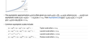
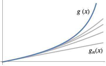
- 如果精确结果为 g[x],x0 处的 n 阶渐近逼近为 gn[x],那么当 xx0 时,AsymptoticLess[g[x]-gn[x],gn[x]-gn-1[x],xx0] 或 g[x]-gn[x]∈o[gn[x]-gn-1[x]].
- 常见的渐近尺度包括:
- 渐近逼近 gn[x] 常以和 gn[x]
αkϕk[x] 的形式给出,其中 {ϕ1[x],…,ϕn[x]} 是当 xx0 时的渐近尺度 ϕ1[x]≻ϕ2[x]≻⋯>ϕn[x]. 当 xx0 时,结果为 AsymptoticLess[g[x]-gn[x],ϕn[x],xx0] 或 g[x]-gn[x]∈o[ϕn[x]]. -

Taylor 尺度,当 xx0 时 
Laurent 尺度,当 xx0 时 
Laurent 尺度,当 x±∞ 时 

Puiseux 尺度,当 xx0 时 - 用于表示渐近逼近的尺度是从问题中自动推断出来的,通常可以包含更多的奇异尺度.
- 可以给出以下选项:
-
AccuracyGoal Automatic 寻求的绝对准确度 Assumptions $Assumptions 对参数的设定 GenerateConditions Automatic 是否给出与参数的条件有关的答案 GeneratedParameters None 怎样命名生成的参数 Method Automatic 所用的方法 PerformanceGoal $PerformanceGoal 优化的目标 PrecisionGoal Automatic 寻求的精度 SeriesTermGoal Automatic 近似式的项数 WorkingPrecision Automatic 内部计算使用的精度 - 当 GenerateConditions 采用默认设置 Automatic 时,Asymptotic 返回的结果中通常不包含参数的条件. 通过将 GenerateConditions 设为 True 可返回包含参数条件的答案.
- PerformanceGoal 的可能设置包括 $PerformanceGoal、"Quality" 和 "Speed". 当设置为 "Quality" 时,Asymptotic 通常可以解出更多的问题或者产生更简单的结果,但是可能会耗费更多的时间和内存. .
- 当 WorkingPrecision、AccuracyGoal 和 PrecisionGoal 采用默认设置 Automatic 时,Asymptotic 可能返回精度较低的渐近逼近,即使输入具有无限精度.
范例
打开所有单元 关闭所有单元基本范例 (4)
求 Sin 在 0 处的渐近逼近的首项:
Asymptotic[Sin[x], x -> 0]Plot[{Sin[x], x}, {x, -2π, 2π}, PlotLegends -> "Expressions"]用 SeriesTermGoal 获取更好的近似:
Asymptotic[Sin[x], x -> 0, SeriesTermGoal -> 12]Plot[Evaluate[{Sin[x], %}], {x, -2π, 2π}, PlotLegends -> "Expressions"]Asymptotic[Integrate[x ^ x, x], x -> 0]用 AsymptoticIntegrate 获得相同的结果:
AsymptoticIntegrate[x ^ x, x, x -> 0]Asymptotic[InverseLaplaceTransform[1 / (s Sqrt[s ^ 3 + 1]), s, t], t -> 0]Asymptotic[DSolveValue[{y''[x] - y'[x] + x^10 y[x] == 1, y[0] == 1, y'[0] == -3 / 4 }, y[x], x], {x, 0, 5}]用 AsymptoticDSolveValue 获得相同的结果:
AsymptoticDSolveValue[{y''[x] - y'[x] + x^10 y[x] == 1, y[0] == 1, y'[0] == -3 / 4 }, y[x], {x, 0, 5}]范围 (36)
初等函数 (8)
多项式在 Infinity 附近渐近逼近的首项:
Asymptotic[x ^ 4 + 5x ^ 3 + 3x - 11, x -> ∞]Plot[{x ^ 4 + 5x ^ 3 + 3x - 11, x ^ 4}, {x, 1, 20}]Asymptotic[(3x ^ 2 + 5) / (4x ^ 2 + 11), x -> ∞]Asymptotic[(3x ^ 3 + 5) / (x ^ 2 - 1), x -> 1]Asymptotic[(3x + 5) / (x ^ 2 + 1) ^ 2, x -> I]Asymptotic[2 ^ x, x -> ∞]Asymptotic[2 ^ x + 3 ^ (-x), x -> 0]Asymptotic[E^x (E^E^-x^2 + E^-x + (1/x) - E^(1/x) - E^-x^2), x -> ∞]Asymptotic[(x ^ 2 + 3x) 2 ^ x, x -> ∞]Asymptotic[(1 / x ^ 2 + 3x)5 ^ (-x), x -> ∞]Asymptotic[(5x ^ 2 / (3x ^ 2 + 1))2 ^ x, x -> ∞]Asymptotic[(5x ^ 2 / (3x ^ 3 + 1))2 ^ x, x -> 0]Asymptotic[Sinh[x], x -> 0]Asymptotic[Sech[x], x -> 0]Asymptotic[ArcSinh[x], x -> 1 / 2]Asymptotic[Log[(x ^ 2 + 1) / (x ^ 2 + 2x)], x -> 0]Asymptotic[(5x ^ 2 / (3x ^ 3 + 1))Log[x], x -> ∞]Asymptotic[(5x ^ 4 / (3x ^ 3 + 1))Log[(3 ^ x + 1)], x -> ∞]Asymptotic[x 2 ^ x, x -> 0]Asymptotic[2 ^ x / (1 + x 2 ^ x), x -> 0]Asymptotic[4 ^ x / (1 + 2 ^ x), x -> ∞]Asymptotic[2 ^ x / (1 + 4 ^ x), x -> ∞]特殊函数 (8)
Gamma 的渐近逼近的首项:
Asymptotic[Gamma[x], x -> ∞]Plot[{Gamma[x], %}//Evaluate, {x, 2, 7}, PlotLegends -> "Expressions"]涉及 Gamma 的复合函数的渐近逼近的首项:
Asymptotic[Gamma[Sin[x] - x + x ^ 3 / 6] ^ 10, x -> 0]Asymptotic[AiryAi[x], x -> ∞]Plot[{AiryAi[x], (E^-(2 x^3 / 2/3)/2 Sqrt[π] x^1 / 4)}, {x, -5, 5}, PlotLegends -> "Expressions"]Asymptotic[AiryBi[x], x -> ∞]Asymptotic[BesselJ[2, x], x -> 0]Asymptotic[BesselJ[2, x], x -> ∞]Plot[{BesselJ[2, x], %}//Evaluate, {x, -5, 20}, PlotLegends -> "Expressions"]Asymptotic[Hypergeometric2F1[1 / 2, 3, a, x], x -> 0]Asymptotic[Hypergeometric2F1[1 / 2, 3, 4, x], x -> 1]Asymptotic[EllipticK[k], k -> 0]Asymptotic[EllipticK[k ^ 2], k -> 1]ReImPlot[{EllipticK[k ^ 2], %}, {k, 0.9, 1.2}, PlotRange -> All]涉及 HarmonicNumber 的函数:
Asymptotic[HarmonicNumber[x], x -> 0]Asymptotic[HarmonicNumber[x] / (x ^ 2 + 1), x -> ∞]涉及 PolyGamma 的函数:
Asymptotic[PolyGamma[x], x -> 0]Asymptotic[E ^ E ^ PolyGamma[PolyGamma[x]] / x, x -> ∞]//FullSimplifyQPolyGamma 的渐近级数:
Asymptotic[QPolyGamma[x, q], x -> 0, SeriesTermGoal -> 3]terms = Table[Asymptotic[QPolyGamma[x, 1 / 3], x -> 0, SeriesTermGoal -> m], {m, 1, 3}];
Plot[{QPolyGamma[x, 1 / 3], terms}, {x, 0, 5}, PlotRange -> {-10, 10}, PlotLegends -> "Expressions"]幂级数表示 (3)
Asymptotic[1 / (1 - x), {x, 0, Infinity}]Asymptotic[1 / (1 - x), {x, 0, Infinity}, GenerateConditions -> True]Asymptotic[Sin[x], {x, 0, Infinity}]TruncateSum[%, 7]使用 Asymptotic 可获得同样的结果:
Asymptotic[Sin[x], {x, 0, 13}]Asymptotic[E ^ x, {x, 1, Infinity}]积分 (2)
Asymptotic[Integrate[Cos[x]E ^ (-x ^ 5 + x), x], x -> 0]AsymptoticIntegrate 获取相同的结果:
AsymptoticIntegrate[Cos[x] E ^ (-a x ^ 5 + x), x, x -> 0]计算 Inactive 定积分的首项:
aint = Asymptotic[Inactive[Integrate][Log[x] * Exp[-x ^ 2], {x, 0, a}], a -> Infinity]N[%]给出从 0 到 Infinity 积分的结果:
int = Integrate[Log[x] * Exp[-x ^ 2], {x, 0, Infinity}]N[%]FullSimplify[aint - int]积分变换 (13)
Asymptotic[Inactive[LaplaceTransform][1 / (E ^ (t ^ 2) + t ^ 17), t, s], s -> Infinity]% /. {s -> 270.}NIntegrate[1 / (E ^ (t ^ 2) + t ^ 17) * E ^ (-270 t), {t, 0, ∞}]Asymptotic[Inactive[InverseLaplaceTransform][1 / Sqrt[s ^ 5 + 1], s, t], t -> 0]Asymptotic[Inactive[MellinTransform][E ^ (-x), x, s], s -> Infinity]Asymptotic[Inactive[InverseMellinTransform][Gamma[s], s, x], x -> 0]Asymptotic[Inactive[FourierTransform][E ^ (-t ^ 2 - t ^ 4), t, x], x -> 0]Asymptotic[Inactive[InverseFourierTransform][t E ^ (-t ^ 2), t, x], x -> 0]Asymptotic[Inactive[FourierSinTransform][E ^ (-t ^ 3), t, x], x -> 0]Asymptotic[Inactive[InverseFourierSinTransform][E ^ (-t ^ 34), t, x], x -> 0]Asymptotic[Inactive[FourierCosTransform][E ^ (-t ^ 3), t, x], x -> 0]Asymptotic[Inactive[InverseFourierCosTransform][3 ^ (-t), t, x], x -> 0]Asymptotic[Inactive[HankelTransform][E ^ (-r), r, s], s -> 0]Asymptotic[Inactive[InverseHankelTransform][E ^ (-3r), r, s], s -> 0]f[x_] := E ^ (-x ^ 2)g[x_] := E ^ (-x ^ 2 - x)Asymptotic[Inactive[Convolve][f[x], g[x], x, y], y -> 0]微分方程 (2)
Asymptotic[DSolveValue[{y''[x] - Cos[x ^ 2] y[x] == 0, y[0] == 3, y'[0] == 2}, y, x], x -> 0]用 AsymptoticDSolveValue 获取相同的结果:
AsymptoticDSolveValue[{y''[x] - Cos[x ^ 2] y[x] == 0, y[0] == 3, y'[0] == 2}, y, x -> 0]计算 DifferentialRoot 的渐近解的首项:
dr = DifferentialRootReduce[E ^ (-x ^ 2 + x), x]Asymptotic[dr, x -> 0, SeriesTermGoal -> 3]选项 (1)
SeriesTermGoal (1)
默认情况下,Asymptotic 返回函数的渐近展开式的首项:
Asymptotic[x E ^ x, x -> 0]Asymptotic[x E ^ x, x -> 0, SeriesTermGoal -> 1]用 SeriesTermGoal 获取更多的项:
Asymptotic[x E ^ x, x -> 0, SeriesTermGoal -> 10]应用 (6)
f[x_] := 2x ^ 2 / (x ^ 2 + 4)asyinf = Asymptotic[f[x], x -> ∞]Plot[{f[x], asyinf}//Evaluate, {x, 0, 7}, PlotLegends -> "Expressions"]比较函数在 0 和 Infinity 处的极限行为:
f[x_] := x + 1 / xasy0 = Asymptotic[f[x], x -> 0]asyinf = Asymptotic[f[x], x -> ∞]Plot[{f[x], asy0, asyinf}//Evaluate, {x, 0, 4}, PlotLegends -> "Expressions"]int = Asymptotic[Inactive[Integrate][1 / Sqrt[1 - ϵ t ^ 14], {t, 0, 1}], ϵ -> 0, SeriesTermGoal -> 3]int /. {ϵ -> 0.3}NIntegrate[1 / Sqrt[1 - 0.3 t ^ 14], {t, 0, 1}]eqn = {y''[x] - 2 y[x] == 0, y[0] == 1, y'[0] == 0};sol = DSolveValue[eqn, y[x], x]//Expandasym = Asymptotic[sol, x -> ∞]Plot[{sol, asym}//Evaluate, {x, 0, 1.2}, PlotLegends -> Automatic]Asymptotic[Sin[Pi z ^ 3 / 2] / (z ^ 5(z - 1)), z -> 1]Asymptotic[Sin[Pi z ^ 3 / 2] / (z ^ 5(z - 1)), z -> 0]ComplexPlot3D[Sin[Pi z ^ 3 / 2] / (z ^ 5(z - 1)), {z, -1 / 2 - 1 / 2I, 3 / 2 + 1 / 2I}, PlotLegends -> Automatic]Asymptotic[PrimePi[x], x -> ∞]Grid[Prepend[Table[{x, N[(x/Log[x])], PrimePi[x]}, {x, 10^Range[8]}], {...}], IconizedObject[«Grid options»]]属性和关系 (6)
Asymptotic 返回的结果渐近等价于输入:
Asymptotic[Sin[x], x -> 0]用 AsymptoticEquivalent 验证结果:
AsymptoticEquivalent[Sin[x], x, x -> 0]Asymptotic 的结果等于该点处的极限,如果极限存在的话:
Asymptotic[Cos[x] + x, x -> 0]Limit[Cos[x] + x, x -> 0]Asymptotic 通常给出级数展开式的首项:
Asymptotic[E ^ (-x ^ 2) Sin[x], x -> 0]Series[E ^ (-x ^ 2) Sin[x], {x, 0, 1}]//NormalAsymptotic 计算连续变量函数的近似值:
Asymptotic[PrimePi[x], x -> ∞]DiscreteAsymptotic 计算离散变量函数的近似值:
DiscreteAsymptotic[PartitionsP[n], n -> ∞]用 AsymptoticExpectation 求期望值的渐近逼近:
dist[b_] := ExponentialDistribution[b];AsymptoticExpectation[E ^ (-x ^ 3), xdist[b], {b, 0, 6}]用 Asymptotic 获取渐近逼近:
Expectation[E ^ (-x ^ 3), xdist[b]]Asymptotic[%, {b, 0, 6}]用 AsymptoticProbability 求概率的渐近逼近:
dist[b_] := ExponentialDistribution[b];AsymptoticProbability[E ^ (x ^ 2 - x) > 3, xdist[b], {b, 0, 2}]用 Asymptotic 获取渐近逼近:
Probability[E ^ (x ^ 2 - x) > 3, xdist[b]]Asymptotic[%, {b, 0, 2}]相关指南
-
▪
- 渐近
文本
Wolfram Research (2020),Asymptotic,Wolfram 语言函数,https://reference.wolfram.com/language/ref/Asymptotic.html (更新于 2022 年).
CMS
Wolfram 语言. 2020. "Asymptotic." Wolfram 语言与系统参考资料中心. Wolfram Research. 最新版本 2022. https://reference.wolfram.com/language/ref/Asymptotic.html.
APA
Wolfram 语言. (2020). Asymptotic. Wolfram 语言与系统参考资料中心. 追溯自 https://reference.wolfram.com/language/ref/Asymptotic.html 年
BibTeX
@misc{reference.wolfram_2026_asymptotic, author="Wolfram Research", title="{Asymptotic}", year="2022", howpublished="\url{https://reference.wolfram.com/language/ref/Asymptotic.html}", note=[Accessed: 08-September-2026]}
BibLaTeX
@online{reference.wolfram_2026_asymptotic, organization={Wolfram Research}, title={Asymptotic}, year={2022}, url={https://reference.wolfram.com/language/ref/Asymptotic.html}, note=[Accessed: 08-September-2026]}