


AudioPlot
Details and Options
- AudioPlot returns a single graphic showing the waveform corresponding to channels of audio.
- AudioPlot has the same options as Graphics, with the following additions and changes: [List of all options]
-
Appearance Automatic appearance of the plot AspectRatio 1/6 the aspect ratio of the plot Axes {True,False} whether to draw axes AxesOrigin {0,0} where axes should cross ColorFunction Automatic how to determine the coloring of waveforms ColorFunctionScaling False whether to scale color function arguments Frame True whether to put a frame around the plot MaxPlotPoints Automatic maximum number of samples to show PlotLayout Automatic the layout to be used PlotRange Automatic range of values to include PlotRangeClipping True whether to clip at the plot range PlotStyle Automatic the styles in which objects are to be drawn PlotTheme $PlotTheme overall theme for the plot - Possible settings for the Appearance option include:
-
"Continuous" continuous plot 
"Discrete" discrete plot 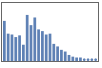
"ContinuousAbs" continuous plot of absolute values 
"DiscreteAbs" discrete plot of absolute values - The plot layout can be specified as PlotLayout->{individual,combination}, where individual specifies the layout for each audio object, and combination specifies how to combine multiple audio objects.
- Possible settings for individual include:
-
"Averaged" waveform of the average of the channels 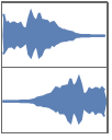
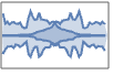
"Overlaid" overlaid waveforms of the channels 
"Vertical" waveform of channels in a vertical grid - Possible settings for combination layouts include:
-
"Overlaid" overlaid waveforms of the audio objects 
"Vertical" grid waveforms of objects in a vertical grid - PlotRange supports the following special settings:
-
t {{0,t},Automatic} plot the first t seconds {t1,t2} {{t1,t2},Automatic} plot the waveform from t1 to t2 seconds - The time specification ti can also be a time quantity (e.g. Quantity[0.1,"Minutes"]) or sample quantity (e.g. Quantity[1000,"Samples"]).
- ColorData["DefaultPlotColors"] gives the default sequence of colors used by PlotStyle.
List of all options
Examples
open all close allBasic Examples (3)
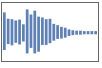
Waveform of a mono audio object:
AudioPlot[\!\(\*AudioBox[""]\)]Waveform of a stereo audio object:
AudioPlot[\!\(\*AudioBox[""]\)]Waveform of the audio track of a video:
AudioPlot[\!\(\*VideoBox[""]\)]Scope (9)
Basic Uses (4)
mono = AudioGenerator["Sin", .01];
AudioPlot[mono]stereo = ExampleData[{"Sound", "Piano"}, "Audio"];
AudioPlot[stereo]multi = AudioChannelCombine[Table[AudioGenerator[i, .01], {i, {"Sin", "Sawtooth", "Triangle"}}]];
AudioPlot[multi]AudioPlot[{\!\(\*AudioBox[""]\), \!\(\*AudioBox[""]\)}]Presentation (5)
Plot the waveform without any frame or axes:
a = Import["ExampleData/rule30.wav"];
AudioPlot[a, Appearance -> "Discrete", Frame -> None, Axes -> None, PlotRange -> All]a = Import["ExampleData/rule30.wav"];
AudioPlot[a, PlotStyle -> RGBColor[0, 2/3, 0], PlotRange -> All]a = Import["ExampleData/rule30.wav"];
AudioPlot[a, PlotTheme -> "Marketing", PlotRange -> All]Add an epilog to the audio plot:
a = ExampleData[{"Sound", "Piano"}, "Audio"];
AudioPlot[a, Epilog -> {Dashed, Red, Line[{{1, -1}, {1, 1}}]}]
Color the waveform with the corresponding value of the high-frequency content to localize onsets:
a = Audio["ExampleData/rule30.wav"];hfc = Rescale@AudioLocalMeasurements[a, "HighFrequencyContent"];Quiet@AudioPlot[a, PlotRange -> {All, All}, Appearance -> "DiscreteAbs", ColorFunction -> Function[{x, y}, ColorData["SunsetColors"]@hfc[x]]]Options (37)
Appearance (4)
By default, a continuous waveform is shown for audio objects:
a = Audio["ExampleData/rule30.wav"];
AudioPlot[a, PlotRange -> {All, All}]AudioPlot[a, Appearance -> "Discrete", PlotRange -> {All, All}]Show a discrete plot of absolute values:
AudioPlot[a, Appearance -> "DiscreteAbs", PlotRange -> {All, All}]The appearance elements are applied to channels of multichannel audio objects:
a = ExampleData[{"Sound", "Piano"}, "Audio"];
AudioPlot[a]
Discrete absolute plot for a stereo audio object:
AudioPlot[a, Appearance -> "DiscreteAbs"]Discrete plot for a list of audio objects:
a = ExampleData[{"Sound", "Piano"}, "Audio"];
b = Audio["ExampleData/rule30.wav"];
AudioPlot[{a, b}, Appearance -> "DiscreteAbs"]
It is possible to control the density of vertical bars in the "Discrete" and "DiscreteAbs" visualizations using the MaxPlotPoints option:
a = Audio["ExampleData/rule30.wav"];
AudioPlot[a, Appearance -> "DiscreteAbs", MaxPlotPoints -> 40, PlotRange -> {All, All}]
AspectRatio (1)
AspectRatio controls the aspect ratio of the plot:
mono = Audio["ExampleData/rule30.wav"];
AudioPlot[mono, ImageSize -> Small, AspectRatio -> 1]
With "Vertical" layout, the setting of AspectRatio controls the aspect ratio of each waveform:
stereo = ExampleData[{"Sound", "Piano"}, "AudioFile"];
AudioPlot[stereo, AspectRatio -> 1]
Axes (1)
All the options related to Axes refer to the axes of the plots of the single channels:
mono = Audio["ExampleData/rule30.wav"];
stereo = ExampleData[{"Sound", "Piano"}, "AudioFile"];AudioPlot[mono, Axes -> False]AudioPlot[stereo, Axes -> False]AxesOrigin (1)
AxesOrigin refers to the plots of the single channels:
mono = Audio["ExampleData/rule30.wav"];
stereo = ExampleData[{"Sound", "Piano"}, "AudioFile"];AudioPlot[mono, Axes -> True, AxesOrigin -> {1, .5}]AudioPlot[stereo, Axes -> True, AxesOrigin -> {1, .5}]ColorFunction (5)
Color by a scaled ![]() coordinate and scaled
coordinate and scaled ![]() coordinate, respectively:
coordinate, respectively:
a = AudioGenerator[{"Sawtooth", 2}];
AudioPlot[a, ColorFunction -> Function[{x, y}, Blend[{Red, Green}, x]]]AudioPlot[a, ColorFunction -> Function[{x, y}, Blend[{Red, Green}, y]]]Color a curve red when its absolute ![]() coordinate is above 0.6:
coordinate is above 0.6:
a = AudioGenerator[{"Sawtooth", 2}];AudioPlot[a, ColorFunction -> Function[{x, y}, If[x > .6, Red, Blue]]]ColorFunction can be used to visualize properties of the audio object:
a = ExampleData[{"Audio", "PianoScale"}];Compute the fundamental frequency of the audio object:
f0 = AudioLocalMeasurements[a, "FundamentalFrequency"];Delete the missing values and rescale it between 0 and 1:
f0 = Rescale[TimeSeries[DeleteMissing[f0//Normal, 1, 2]]]Use the result so that the color of the waveform is proportional to the fundamental frequency at that time:
Quiet@AudioPlot[a, ColorFunction -> Function[{x, y}, ColorData["SolarColors"][f0[x]]]]ColorFunction has higher priority than PlotStyle for coloring the waveform:
audio = AudioGenerator[{"Sawtooth", 2}];AudioPlot[audio, ColorFunction -> Function[{x, y}, Hue[x]], PlotStyle -> Orange]ColorFunction can be used with any setting of Appearance:
a = Audio["ExampleData/rule30.wav"];AudioPlot[a, ColorFunction -> Function[{x, y}, Hue[y]], Appearance -> "DiscreteAbs", PlotRange -> {All, All}]ColorFunctionScaling (1)
No argument scaling on the left; automatic scaling on the right:
audio = AudioGenerator[{"Sawtooth", 4}, .5];Table[AudioPlot[audio, ColorFunction -> Function[{x, y}, Blend[{Red, Green}, x]], ColorFunctionScaling -> cf, ImageSize -> Small], {cf, {False, True}}]FillingStyle (2)
a = Audio["ExampleData/car.mp3"];
AudioPlot[a, FillingStyle -> Opacity[.3], MaxPlotPoints -> 200]
Control the filling style channel by channel:
a = ExampleData[{"Audio", "Piano"}];
AudioPlot[a, FillingStyle -> {RGBColor[1, 0.5, 0], RGBColor[0, 2/3, 0]}]
Control the filling style of multiple audio objects:
a1 = Import["ExampleData/rule30.wav"];
a2 = ExampleData[{"Audio", "Piano"}];AudioPlot[{a1, a2}, FillingStyle -> Opacity[.3]]Control the filling style audio by audio:
AudioPlot[{a1, a2}, FillingStyle -> {RGBColor[1, 0.5, 0], RGBColor[0, 2/3, 0]}]Specify the filling style of the channels of each audio object:
AudioPlot[{a1, a2}, FillingStyle -> {{RGBColor[1/3, 1/3, 1]}, {RGBColor[0, 2/3, 0], RGBColor[2/3, 0, 0]}}]FrameTicks (5)
The Automatic setting will generate only two ticks for the ![]() axis independently of PlotRange:
axis independently of PlotRange:
a = Audio["ExampleData/rule30.wav"];AudioPlot[a, FrameTicks -> {None, Automatic}, PlotRange -> {All, All}]It is possible to specify the FrameTicks for each axis:
a = ExampleData[{"Audio", "Piano"}];
AudioPlot[a, FrameTicks -> {{Automatic, All}, {None, All}}]
Place tick marks at specified positions:
a = ExampleData[{"Audio", "Piano"}];yticks = {-.8, 0, .8};AudioPlot[a, FrameTicks -> {{yticks, None}, {None, None}}]Place tick marks at specified positions with arbitrary labels:
a = ExampleData[{"Audio", "Piano"}];yticks = {{-.8, -.8}, {0, "zero"}, {.8, .8}};AudioPlot[a, FrameTicks -> {{yticks, None}, {None, None}}]Specify the ticks as a function:
audio = Import["ExampleData/rule30.wav"];ticks[min_, max_] := Table[i, {i, 0, max, Round[(max - min) / 6, .1]}]AudioPlot[audio, FrameTicks -> {ticks, Automatic}]MaxPlotPoints (1)
MaxPlotPoints controls the maximum number of points displayed:
a = 2.Import["ExampleData/rule30.wav"];AudioPlot[a, MaxPlotPoints -> 5000]The smaller the number of points displayed, the more smoothing is applied:
AudioPlot[a, MaxPlotPoints -> 40]PlotLabel (2)
PlotLayout (3)
Choose among different plot layouts with a multichannel audio object:
a = ExampleData[{"Audio", "Piano"}];AudioPlot[a, PlotLayout -> "Vertical"]AudioPlot[a, PlotLayout -> "Overlaid"]AudioPlot[a, PlotLayout -> "Averaged"]Choose between different plot layouts with a list of audio objects:
a1 = Import["ExampleData/rule30.wav"];
a2 = ExampleData[{"Audio", "Piano"}];AudioPlot[{a1, a2}, PlotLayout -> "Vertical"]AudioPlot[{a1, a2}, PlotLayout -> "Overlaid"]Control the individual and combination layouts independently:
a1 = Import["ExampleData/rule30.wav"];
a2 = ExampleData[{"Audio", "Piano"}];AudioPlot[{a1, a2}, PlotLayout -> {"Overlaid", "Vertical"}, MaxPlotPoints -> 500, PlotLabel -> {"Overlaid", "Vertical"}, PlotRange -> All]AudioPlot[{a1, a2}, PlotLayout -> {"Averaged", "Overlaid"}, MaxPlotPoints -> 500, PlotLabel -> {"Averaged", "Overlaid"}, PlotRange -> All]PlotRange (4)
Plot only the first second of an audio object:
AudioPlot[ExampleData[{"Sound", "Piano"}, "Audio"], PlotRange -> 1]Specify the ![]() range using a time Quantity:
range using a time Quantity:
a = AudioGenerator["Sin", 10];
AudioPlot[a, PlotRange -> Quantity[10, "Milliseconds"]]
Use a "Samples" Quantity:
AudioPlot[a, PlotRange -> Quantity[200, "Samples"]]Plot the waveform between 100 and 120 ms:
a = ExampleData[{"Sound", "Piano"}, "Audio"];
AudioPlot[a, PlotRange -> {Quantity[100, "Milliseconds"], Quantity[120, "Milliseconds"]}]a = ExampleData[{"Sound", "Piano"}, "AudioFile"];
AudioPlot[a, PlotRange -> {Automatic, {0, 1}}]PlotStyle (4)
PlotStyle specifies the style in which the waveform is to be drawn:
a = Audio["ExampleData/rule30.wav"];AudioPlot[a, PlotStyle -> RGBColor[1, 0.5, 0]]AudioPlot[a, PlotStyle -> Directive[RGBColor[0, 0, 1], Opacity[.3]]]Explicitly style each channel:
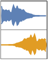
a = ExampleData[{"Audio", "Piano"}];AudioPlot[a, PlotStyle -> {RGBColor[1, 0.5, 0], RGBColor[0, 2/3, 0]}]AudioPlot will automatically style multiple audio objects:
a1 = ExampleData[{"Audio", "Piano"}];
a2 = Audio["ExampleData/rule30.wav"];AudioPlot[{a1, a2}]Control the style of multiple audio objects:
a1 = ExampleData[{"Audio", "Piano"}];
a2 = Audio["ExampleData/rule30.wav"];AudioPlot[{a1, a2}, PlotStyle -> Opacity[.5]]Explicitly style multiple audio objects:
AudioPlot[{a1, a2}, PlotStyle -> {RGBColor[1, 0.5, 0], RGBColor[0, 2/3, 0]}]Specify the style of the individual channels of each audio object:
AudioPlot[{a1, a2}, PlotStyle -> {{RGBColor[0, 2/3, 0], RGBColor[1/3, 1/3, 1]}, {RGBColor[1, 0.5, 0]}}]PlotTheme (3)
Use a theme with simple styling and a bright color scheme:
AudioPlot[ExampleData[{"Audio", "Piano"}], PlotTheme -> "Business"]AudioPlot[ExampleData[{"Audio", "Piano"}], PlotTheme -> "Business", PlotStyle -> ColorData[96]]AudioPlot[ExampleData[{"Audio", "Piano"}], PlotTheme -> "Minimal"]Applications (3)
Highlight parts of an audio object:
a = ExampleData[{"Sound", "FluteScale"}, "Audio"];silence = AudioIntervals[a, "Inaudible", 0.1];
AudioPlot[a, Epilog -> {RGBColor[1, 0, 0, .2], Rectangle[{#[[1]], -1}, {#[[2]], 1}]& /@ silence}]Plot waveforms of audio files in a collection:
Multicolumn[AudioPlot[ExampleData[#, "AudioFile"], PlotLabel -> #[[2]], PlotTheme -> "Minimal"]& /@ ExampleData["Sound"][[ ;; 12]], 3]Show a TimeSeries on top of the waveform:
a = Audio["ExampleData/car.mp3"];ts = AudioLocalMeasurements[a, "RMSAmplitude"];Show[AudioPlot[a], ListLinePlot[ts, PlotStyle -> Pink]]Interactive Examples (1)
Neat Examples (1)
Create a 3D-printable model of the waveform of an audio object:
a = AudioChannelMix[ExampleData[{"Audio", "Drums"}], 1];plot = AudioPlot[a, AspectRatio -> 1 / 3, PlotStyle -> White, Background -> Black, Frame -> False, Axes -> False]RegionProduct[ImageMesh@plot, Line[{{0.}, {20}}]]Printout3D[%, "waveform.stl"]Text
Wolfram Research (2016), AudioPlot, Wolfram Language function, https://reference.wolfram.com/language/ref/AudioPlot.html (updated 2024).
CMS
Wolfram Language. 2016. "AudioPlot." Wolfram Language & System Documentation Center. Wolfram Research. Last Modified 2024. https://reference.wolfram.com/language/ref/AudioPlot.html.
APA
Wolfram Language. (2016). AudioPlot. Wolfram Language & System Documentation Center. Retrieved from https://reference.wolfram.com/language/ref/AudioPlot.html