ComplexContourPlot[f,{z,zmin,zmax}]
f の塗潰し等高線プロットを z の関数として生成する.
ComplexContourPlot[{f1,f2,…},{z,zmin,zmax}]
f1, f2, …の等高線を生成する.
ComplexContourPlot[f==g,{z,zmin,zmax}]
f=g である等高線をプロットする.
ComplexContourPlot[{f1==g1,f2==g2,…},{z,zmin,zmax}]
f1g1, f2=g2, …のそれぞれの等高線をプロットする.
ComplexContourPlot
ComplexContourPlot[f,{z,zmin,zmax}]
f の塗潰し等高線プロットを z の関数として生成する.
ComplexContourPlot[{f1,f2,…},{z,zmin,zmax}]
f1, f2, …の等高線を生成する.
ComplexContourPlot[f==g,{z,zmin,zmax}]
f=g である等高線をプロットする.
ComplexContourPlot[{f1==g1,f2==g2,…},{z,zmin,zmax}]
f1g1, f2=g2, …のそれぞれの等高線をプロットする.
詳細とオプション
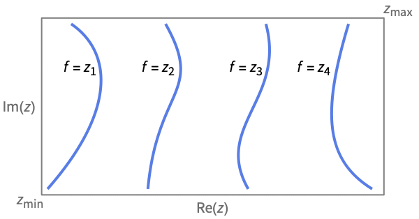
- f を評価しても実数にならないところには,等高線プロットの背景が見えるように穴が残される.関数 f と g は,大抵の場合,比較の目的で複素数から実数部分を抽出するRe,Im,Abs,Argのような関数を含む.
- ComplexContourPlot[f,{z,n}]はComplexContourPlot[f,{z,-n-n I,n+n I}]に等しい.
- ComplexContourPlotは,事実上Blockを使って,変数 z を局所的なものとして扱う.
- ComplexContourPlotには属性HoldAllがあり,z に特定の数値を割り当てた後ではじめて fiと giを評価する.場合によっては,Evaluateを使ってまず f と g を記号的に評価した方が効率的かもしれない.
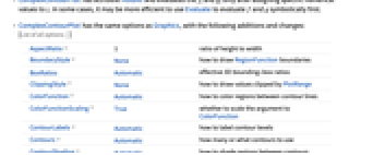
- ComplexContourPlotにはGraphics,と同じオプションに以下の追加・変更を加えたものが使える. [全オプションのリスト]
- 次は,PlotLegendsでよく使われる設定である.
-
None 凡例は使わない Automatic 凡例を自動的に決定する Placed[lspec,…] 凡例の置き方を指定する - ContourShading->Automaticのデフォルト設定では,ComplexContourPlot[f,…]については陰影付けが行われるが,ComplexContourPlot[f=g,…]やComplexContourPlot[{f1,f2,…},…]については行われない.
- ComplexContourPlot[{f1==g1,f2==g2,…},…]は,等式 fi==gi のすべてに関連する等高線を重ね合せる.
- 等高線レベル間の領域の彩色方法の決定の際,ComplexContourPlotは,まずContourShadingに与えられた明示的な設定を調べて,その後ColorFunctionに与えられた設定を調べる.
- ComplexContourPlot[{f1,f2,…},…]で複数の関数の等高線をプロットするときは,等高線指定のリストContours{spec1,spec2,…}で各 fiについての対応する speciが使われる.
- ColorData["DefaultPlotColors"]は,ContourStyleで使われるデフォルトの色のシーケンスを与える.
- ComplexContourPlotは,まず,PlotPointsで指定された等間隔のサンプル点の格子で f を評価する.次に,適応的アルゴリズムを使って最高でMaxRecursion回再分割してなめらかな等高線を生成する.
- 有限個のサンプル点しか使わないので,ComplexContourPlotが関数特徴を見逃す可能性があるので注意が必要である.結果のチェックには,PlotPointsとMaxRecursionの設定を大きくするとよい.
- PerformanceGoalの何らかの設定で他の明示的なオプション設定が上書きされることがある.
- MeshFunctionsとRegionFunctionの中の関数に渡される引数は z と f である.
- ColorFunctionには引数が1つ渡される.この引数はデフォルトで,連続する等高線レベルの各ペアについての f のスケールされた値の平均で渡される.
- デフォルト設定のExclusions->AutomaticおよびExclusionsStyle->Noneでは,不連続性を感知した位置で,ContourPlotのサンプリングの連続性が途絶える.この不連続性は,特定の等高レベルから飛び抜けるような場合にのみ即座に分かるようになる.
- 次は,ScalingFunctionsの可能な設定である.
-
sf f の値をスケールする {sRe,sIm} 実軸と虚軸をスケールする {sRe,sIm,sf} 実軸,虚軸,f の値をスケールする
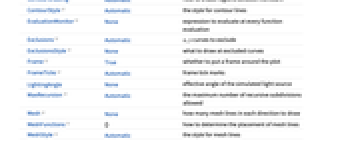
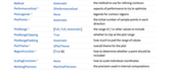
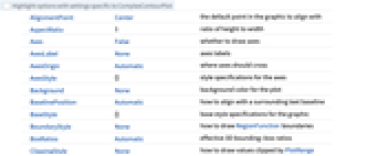
全オプションのリスト
例題
すべて開く すべて閉じる例 (4)
ComplexContourPlot[Abs[z], {z, -3 - 3I, 3 + 3I}]ComplexContourPlot[Re[z] == Im[1 / z], {z, 2}]ComplexContourPlot[{Re[z], Im[1 / z]}, {z, 2}]ComplexContourPlot[{Abs[z] == Re[z] + 1, Abs[z] == Re[z] + 2, Abs[z] == Re[z] + 3}, {z, -3 - 3I, 3 + 3I}, PlotLegends -> "Expressions"]スコープ (18)
サンプリング (6)
関数が急速に変化するところではより多くの点がサンプルとして取られる:
ComplexContourPlot[Abs[z^2 + 1], {z, 0, 2 + 2I}, Mesh -> All]白い部分は関数が切り取られたことを示す.プロット範囲は自動的に選択される:
ComplexContourPlot[Abs[1 / z], {z, -3 - 3I, 3 + 3I}]PlotRangeを使って関心領域に焦点を当てる:
ComplexContourPlot[Abs[1 / z], {z, -3 - 3I, 3 + 3I}, PlotRange -> {0.2, 5}]PlotPointsとMaxRecursionを使って適応的サンプリングを制御する:
Table[ComplexContourPlot[Abs[Sin[z^1 / 2] + 1], {z, 0, 2 + 2I}, PlotPoints -> pp, MaxRecursion -> mr], {mr, {0, 2}}, {pp, {5, 15}}]RegionFunctionを使って不等式が与える領域に曲面を限定する:
ComplexContourPlot[Re[ArcSin[z]], {z, -3 - 3I, 3 + 3I}, RegionFunction -> Function[{z, f}, Abs[z] < 3]]Exclusionsを使って不連続性を切断するかどうか,また,どこで切断するかを制御する:
{ComplexContourPlot[Arg[ArcSin[z^2]], {z, -3 - 3I, 3 + 3I}],
ComplexContourPlot[Arg[ArcSin[z^2]], {z, -3 - 3I, 3 + 3I}, Exclusions -> None]}ラベルと凡例 (6)
ComplexContourPlot[Re[Sqrt[z]], {z, -3 - 3I, 3 + 3I}, FrameLabel -> {Re[z], Im[z]}, PlotLabel -> Re[Sqrt[z]]]ComplexContourPlot[Re[Sqrt[z]] == 1, {z, -3 - 3I, 3 + 3I}, FrameLabel -> {Re[z], Im[z]}, PlotLabel -> Re[Sqrt[z]] == 1]ComplexContourPlot[Re[Sqrt[z]], {z, -3 - 3I, 3 + 3I}, ContourLabels -> True]ComplexContourPlot[Re[Sqrt[z]], {z, -3 - 3I, 3 + 3I}, PlotLegends -> Automatic]ComplexContourPlot[ReIm[Sqrt[z]], {z, -3 - 3I, 3 + 3I}, PlotLegends -> "Expressions"]複数の関数については,線の凡例をプレースホルダと一緒に使う:
ComplexContourPlot[ReIm[Sqrt[z]], {z, -3 - 3I, 3 + 3I}, PlotLegends -> Automatic]ComplexContourPlot[{Re[z^2] == 1, Im[z^2] == 1}, {z, -3 - 3I, 3 + 3I}, PlotLegends -> "Expressions"]プレゼンテーション (6)
ComplexContourPlot[Re[Sqrt[z]], {z, -3 - 3I, 3 + 3I}, ColorFunction -> "Rainbow"]ComplexContourPlot[Re[z^2], {z, -3 - 3I, 3 + 3I}, ContourShading -> Hue /@ Range[0, 1, 0.1]]ComplexContourPlot[Re[z^2], {z, -3 - 3I, 3 + 3I}, ContourStyle -> {Red, Directive[Red, Dashed]}]ComplexContourPlot[{Re[z^2] == 1, Im[z^2] == 1}, {z, -3 - 3I, 3 + 3I}, ContourStyle -> {Green, Dashed}]ComplexContourPlot[Re[z^2], {z, -3 - 3I, 3 + 3I}, Mesh -> 10, MeshFunctions -> {Re[#1]&, Im[#1]&}]ComplexContourPlot[Re[z^2], {z, -3 - 3I, 3 + 3I}, PlotTheme -> "Scientific"]オプション (138)
AspectRatio (4)
デフォルトで,AspectRatioは幅と長さに同じ長さを使う:
ComplexContourPlot[Abs[z^2 - 2], {z, -4 - 2I, 4 + 2I}]ComplexContourPlot[Abs[z^2 - 2], {z, -4 - 2I, 4 + 2I}, AspectRatio -> 1 / 2]AspectRatioAutomaticはプロット範囲から縦横比を決定する:
ComplexContourPlot[Abs[z^2 - 2], {z, -4 - 2I, 4 + 2I}, AspectRatio -> Automatic]AspectRatioFullは他の構造物にぴったり収まるように縦横を調整する:
plot = ComplexContourPlot[Abs[z^2 - 2], {z, -4 - 2I, 4 + 2I}, AspectRatio -> Full];{Framed[Pane[plot, {240, 200}]], Framed[Pane[plot, {230, 230}]]}Axes (4)
デフォルトで,ComplexContourPlotは軸の代りに枠を使う:
ComplexContourPlot[Abs[Sin[z^1 / 2 - 3]], {z, -4 - 4I, 4 + 4I}]ComplexContourPlot[Abs[Sin[z^1 / 2 - 3]], {z, -4 - 4I, 4 + 4I}, Frame -> False, Axes -> True]AxesOriginを使って軸の交点を指定する:
ComplexContourPlot[Abs[Sin[z^1 / 2 - 3]], {z, -4 - 4I, 4 + 4I}, Frame -> False, Axes -> True, AxesOrigin -> {0, 0}]{ComplexContourPlot[Abs[Sin[z^1 / 2 - 3]], {z, -4 - 4I, 4 + 4I}, Frame -> False, Axes -> {True, False}], ComplexContourPlot[Abs[Sin[z^1 / 2 - 3]], {z, -4 - 4I, 4 + 4I}, Frame -> False, Axes -> {False, True}]}AxesLabel (3)
ComplexContourPlot[Abs[Sin[z^1 / 2 - 3]], {z, -4 - 4I, 4 + 4I}, Frame -> False, Axes -> True]ComplexContourPlot[Abs[Sin[z^1 / 2 - 3]], {z, -4 - 4I, 4 + 4I}, Frame -> False, Axes -> True, AxesLabel -> Y]ComplexContourPlot[Abs[Sin[z^1 / 2 - 3]], {z, -4 - 4I, 4 + 4I}, Frame -> False, Axes -> True, AxesLabel -> {"X", "Y"}]AxesOrigin (2)
AxesStyle (4)
ComplexContourPlot[Abs[Sin[z^1 / 2 - 3]], {z, -4 - 4I, 4 + 4I}, Frame -> False, Axes -> True, AxesStyle -> Red]ComplexContourPlot[Abs[Sin[z^1 / 2 - 3]], {z, -4 - 4I, 4 + 4I}, Frame -> False, Axes -> True, AxesStyle -> {{Thick, Red}, {Thick, Blue}}]ComplexContourPlot[Abs[Sin[z^1 / 2 - 3]], {z, -4 - 4I, 4 + 4I}, Frame -> False, Axes -> True, AxesStyle -> Green, TicksStyle -> Black]ComplexContourPlot[Abs[Sin[z^1 / 2 - 3]], {z, -4 - 4I, 4 + 4I}, Frame -> False, Axes -> True, AxesStyle -> Green, LabelStyle -> Black]BoundaryStyle (3)
ComplexContourPlot[Abs[Sin[z^1 / 2 - 3]], {z, -4 - 4I, 4 + 4I}, BoundaryStyle -> Red]BoundaryStyleはRegionFunctionで切り取られた穴の周りに適用されるが,Exclusionsで切り取られた部分の周りには適用されない:
ComplexContourPlot[Abs[Sin[z^1 / 2 - 3]], {z, -4 - 4I, 4 + 4I}, BoundaryStyle -> Red, RegionFunction -> Function[{z, f}, Abs[z] > 2]]代りにExclusionsStyleを使う:
ComplexContourPlot[Abs[Sin[z^1 / 2 - 3]], {z, -4 - 4I, 4 + 4I}, ExclusionsStyle -> Red]ClippingStyle (4)
ComplexContourPlot[Re[Exp[I z^2]], {z, -3 - 3I, 3 + 3I}, ClippingStyle -> Automatic]ComplexContourPlot[Re[Exp[I z^2]], {z, -3 - 3I, 3 + 3I}, ClippingStyle -> None]ComplexContourPlot[Re[Exp[I z^2]], {z, -3 - 3I, 3 + 3I}, ClippingStyle -> Pink]曲面の上が切り取られた部分に緑を,下が切り取られた部分に赤を使う:
ComplexContourPlot[Re[Exp[I z^2]], {z, -3 - 3I, 3 + 3I}, ClippingStyle -> {Pink, Green}]ColorFunction (3)
ComplexContourPlot[Abs[Sin[z^1 / 2 - 3]], {z, -4 - 4I, 4 + 4I}, ColorFunction -> Hue]ComplexContourPlot[Abs[Sin[z^1 / 2 - 3]], {z, -4 - 4I, 4 + 4I}, ColorFunction -> "WatermelonColors"]ComplexContourPlot[Abs[Sin[z^1 / 2 - 3]], {z, -4 - 4I, 4 + 4I}, ColorFunction -> (If[#1 > 1, Red, White]&), ColorFunctionScaling -> False]ColorFunctionScaling (1)
ColorFunctionはスケールされた座標にもスケールされていない座標にも使える:
Table[ComplexContourPlot[Abs[z], {z, -2 - 2I, 2 + 2I}, Contours -> 20, ColorFunction -> Hue, ColorFunctionScaling -> cf], {cf, {True, False}}]ContourLabels (2)
ComplexContourPlot[Arg[Sec[z]], {z, -π - π I, π + π I}, ContourLabels -> True]ComplexContourPlot[Arg[Sec[z]], {z, -π - π I, π + π I}, ContourLabels -> Function[{x, y, z}, Text[Framed[z], {x, y}, Background -> StandardGray]]]Contours (9)
ComplexContourPlot[Im[z^3 + 1], {z, -1 - 1I, 1 + 1I}, Contours -> 10]ComplexContourPlot[Im[z^3 + 1], {z, -1 - 1I, 1 + 1I}, Contours -> Automatic]ComplexContourPlot[Im[z^3 + 1], {z, -1 - 1I, 1 + 1I}, Contours -> {Automatic, 5}]ComplexContourPlot[Im[z^3 + 1], {z, -1 - 1I, 1 + 1I}, Contours -> {-0.5, 0, 0.5}]ComplexContourPlot[Im[z^3 + 1], {z, -1 - 1I, 1 + 1I}, Contours -> {{-0.5, Red}, {0, Green}, {0.5, Blue}}]ComplexContourPlot[Im[z^3 + 1], {z, -1 - 1I, 1 + 1I}, Contours -> Function[{min, max}, Range[min, max, 0.1]]]ComplexContourPlot[Im[z^3 + 1], {z, -1 - 1I, 1 + 1I}, Contours -> Function[{min, max}, Rescale[{0.4, 0.8}, {0, 1}, {min, max}]]]複数の関数が指定されたときは,等高線の本数を個別に制御することができる:
ComplexContourPlot[ReIm[z^3 + 1], {z, -1 - 1I, 1 + 1I}, Contours -> {5, 10}]ComplexContourPlot[ReIm[z^3 + 1], {z, -1 - 1I, 1 + 1I}, Contours -> {Range[0, 1, 0.2], Range[0, 2, 0.1]}]ContourShading (5)
ComplexContourPlot[Im[z^3 + 1], {z, -1 - 1I, 1 + 1I}, ContourShading -> Automatic]Noneを使って等高線だけを示す:
ComplexContourPlot[Im[z^3 + 1], {z, -1 - 1I, 1 + 1I}, ContourShading -> None]関数のリストが指定されたときは,陰影付けは自動的にオフになる:
ComplexContourPlot[ReIm[Sqrt[z]], {z, -3 - 3I, 3 + 3I}]ComplexContourPlot[Im[z^3 + 1], {z, -1 - 1I, 1 + 1I}, ContourShading -> Automatic, ColorFunction -> "Rainbow"]ComplexContourPlot[Im[z^3 + 1], {z, -1 - 1I, 1 + 1I}, Contours -> 3, ContourShading -> {Red, Orange, Yellow, White}]ContourStyle (7)
ComplexContourPlot[Im[z^3 + 1], {z, -1 - 1I, 1 + 1I}, ContourStyle -> Automatic]ComplexContourPlot[Im[z^3 + 1], {z, -1 - 1I, 1 + 1I}, ContourStyle -> Directive[Dashed, Opacity[1]]]Noneを使って等高線が描かれないようにする:
ComplexContourPlot[Im[z^3 + 1], {z, -1 - 1I, 1 + 1I}, ContourStyle -> None]ContourStyleNoneはContourLinesFalseに等しい:
ComplexContourPlot[Im[z^3 + 1], {z, -1 - 1I, 1 + 1I}, ContourLines -> False, ContourStyle -> Black]ComplexContourPlot[Im[z^3 + 1], {z, -1 - 1I, 1 + 1I}, ContourStyle -> {Red, Dashed}]ComplexContourPlot[{Abs[z^2 + 1], Abs[z^2 - 1]}, {z, -2 - 2I, 2 + 2I}, ContourStyle -> {Red, Blue}]ComplexContourPlot[{Abs[z^3 + 1] == 2, Abs[z^3 - 1] == 2}, {z, -2 - 2I, 2 + 2I}, ContourStyle -> {Red, Dashed}]ComplexContourPlot[{Abs[z^3 + 1] == 2, Abs[z^3 - 1] == 2}, {z, -2 - 2I, 2 + 2I}, ContourStyle -> Directive[Red, Dashed]]EvaluationMonitor (2)
ContourPlotは関数のサンプルを取っているところを示す:
ComplexListPlot[Reap[ComplexContourPlot[Arg[ArcTan[z]], {z, -2 - 2I, 2 + 2I}, EvaluationMonitor :> Sow[z]]][[-1, 1]], PlotStyle -> PointSize[Tiny]]Block[{k = 0}, ComplexContourPlot[Arg[ArcTan[z]], {z, -2 - 2I, 2 + 2I}, EvaluationMonitor :> k++];k]Exclusions (6)
ComplexContourPlot[Re[ArcCos[z^2]], {z, -3 - 3I, 3 + 3I}]ComplexContourPlot[Re[ArcCos[z^2]], {z, -3 - 3I, 3 + 3I}, Exclusions -> None]ComplexContourPlot[Re[ArcCos[z^2]], {z, -3 - 3I, 3 + 3I}, Exclusions -> Im[z] == 0]ComplexContourPlot[Re[ArcCos[z^2]], {z, -3 - 3I, 3 + 3I}, Exclusions -> {Im[z] == 0, Re[z] == 0}]ComplexContourPlot[Re[ArcCos[z^2]], {z, -3 - 3I, 3 + 3I}, Exclusions -> {{Im[z] == 0, Abs[Re[z]] > 1}, {Re[z] == 0, Abs[Im[z]] > 1}}]ComplexContourPlot[Re[ArcCos[z^2]], {z, -3 - 3I, 3 + 3I}, Exclusions -> {Automatic, Abs[z] == 1}]ExclusionsStyle (2)
Frame (4)
ComplexContourPlotはデフォルトで枠を使う:
ComplexContourPlot[{Abs[z] == Re[z] + 1, Abs[z] == Re[z] + 2, Abs[z] == Re[z] + 3}, {z, -3 - 3 I, 3 + 3 I}]ComplexContourPlot[{Abs[z] == Re[z] + 1, Abs[z] == Re[z] + 2, Abs[z] == Re[z] + 3}, {z, -3 - 3 I, 3 + 3 I}, Frame -> False]ComplexContourPlot[{Abs[z] == Re[z] + 1, Abs[z] == Re[z] + 2, Abs[z] == Re[z] + 3}, {z, -3 - 3 I, 3 + 3 I}, Frame -> {{True, True}, {False, False}}]ComplexContourPlot[{Abs[z] == Re[z] + 1, Abs[z] == Re[z] + 2, Abs[z] == Re[z] + 3}, {z, -3 - 3 I, 3 + 3 I}, Frame -> {{True, False}, {True, False}}]FrameLabel (4)
ComplexContourPlot[{Abs[z] == Re[z] + 1, Abs[z] == Re[z] + 2, Abs[z] == Re[z] + 3}, {z, -3 - 3 I, 3 + 3 I}, FrameLabel -> {"label"}]ComplexContourPlot[{Abs[z] == Re[z] + 1, Abs[z] == Re[z] + 2, Abs[z] == Re[z] + 3}, {z, -3 - 3 I, 3 + 3 I}, FrameLabel -> Automatic]ComplexContourPlot[{Abs[z] == Re[z] + 1, Abs[z] == Re[z] + 2, Abs[z] == Re[z] + 3}, {z, -3 - 3 I, 3 + 3 I}, FrameLabel -> {{"left", "right"}, {"bottom", "top"}}]ComplexContourPlot[{Abs[z] == Re[z] + 1, Abs[z] == Re[z] + 2, Abs[z] == Re[z] + 3}, {z, -3 - 3 I, 3 + 3 I}, FrameLabel -> {{"left", "right"}, {"bottom", "top"}}, LabelStyle -> Directive[Bold, StandardGray]]FrameStyle (2)
ComplexContourPlot[{Abs[z] == Re[z] + 1, Abs[z] == Re[z] + 2, Abs[z] == Re[z] + 3}, {z, -3 - 3 I, 3 + 3 I}, FrameStyle -> Directive[StandardGray, Thick]]ComplexContourPlot[{Abs[z] == Re[z] + 1, Abs[z] == Re[z] + 2, Abs[z] == Re[z] + 3}, {z, -3 - 3 I, 3 + 3 I}, FrameStyle -> {{Directive[Green, Thick], Directive[Red]}, {Directive[Gray, Thick], Directive[Blue]}}]FrameTicks (9)
ComplexContourPlot[{Abs[z] == Re[z] + 1, Abs[z] == Re[z] + 2, Abs[z] == Re[z] + 3}, {z, -3 - 3 I, 3 + 3 I}]ComplexContourPlot[{Abs[z] == Re[z] + 1, Abs[z] == Re[z] + 2, Abs[z] == Re[z] + 3}, {z, -3 - 3 I, 3 + 3 I}, FrameTicks -> None]ComplexContourPlot[{Abs[z] == Re[z] + 1, Abs[z] == Re[z] + 2, Abs[z] == Re[z] + 3}, {z, -3 - 3 I, 3 + 3 I}, FrameTicks -> {{None, None}, {Automatic, None}}]デフォルトで,上と右の辺には目盛は置かれるが目盛ラベルは付けられない:
ComplexContourPlot[{Abs[z] == Re[z] + 1, Abs[z] == Re[z] + 2, Abs[z] == Re[z] + 3}, {z, -3 - 3 I, 3 + 3 I}, FrameTicks -> Automatic]Allを使って目盛ラベルをすべての辺に付ける:
ComplexContourPlot[{Abs[z] == Re[z] + 1, Abs[z] == Re[z] + 2, Abs[z] == Re[z] + 3}, {z, -3 - 3 I, 3 + 3 I}, FrameTicks -> All]ComplexContourPlot[{Abs[z] == Re[z] + 1, Abs[z] == Re[z] + 2, Abs[z] == Re[z] + 3}, {z, -5 - 5 I, 5 + 5 I}, FrameTicks -> {{{1, 3, 5}, {1, 3, 5}}, {{1, 3, 4}, {1, 3, 4}}}]ComplexContourPlot[{Abs[z] == Re[z] + 1, Abs[z] == Re[z] + 2, Abs[z] == Re[z] + 3}, {z, -5 - 5 I, 5 + 5 I}, FrameTicks -> {{{{1, a}, {3, b}, {5, d}}, Automatic}, {{{1, a}, {3, b}, {4, c}}, Automatic}}]ComplexContourPlot[{Abs[z] == Re[z] + 1, Abs[z] == Re[z] + 2, Abs[z] == Re[z] + 3}, {z, -5 - 5 I, 5 + 5 I}, FrameTicks -> {{{{1, a, .37}, {3, b, .5}, {5, d, .75}}, Automatic}, {{{1, a, .13}, {3, b, .12}, {4, c, .2}}, Automatic}}]ComplexContourPlot[{Abs[z] == Re[z] + 1, Abs[z] == Re[z] + 2, Abs[z] == Re[z] + 3}, {z, -5 - 5 I, 5 + 5 I}, FrameTicks -> {{Automatic, Automatic}, {{{1, a, {.13, 0.05}}, {3, b, {.12, .1}}, {4, c, {.2, .2}}}, Automatic}}]ComplexContourPlot[{Abs[z] == Re[z] + 1, Abs[z] == Re[z] + 2, Abs[z] == Re[z] + 3}, {z, -5 - 5 I, 5 + 5 I}, FrameTicks -> {{{{1, a, .37, Directive[Red]}, {3, b, .5, Directive[Red, Thick, Dashed]}, {5, d, .75, Directive[Green, Thick, Dashed]}}, Automatic}, {Automatic, Automatic}}]minMeanMax[min_, max_] := {{min, min}, {(max + min) / 2, (max + min) / 2}, {max, max}}ComplexContourPlot[{Abs[z] == Re[z] + 1, Abs[z] == Re[z] + 2, Abs[z] == Re[z] + 3}, {z, -1 - 1 I, 5 + 5 I}, FrameTicks -> {{minMeanMax, None}, {minMeanMax, None}}, PlotRangePadding -> None]FrameTicksStyle (3)
デフォルトで,目盛と目盛ラベルには枠と同じスタイルが使われる:
ComplexContourPlot[{Abs[z] == Re[z] + 1, Abs[z] == Re[z] + 2, Abs[z] == Re[z] + 3}, {z, -3 - 3 I, 3 + 3 I}, FrameStyle -> Directive[Red]]ComplexContourPlot[{Abs[z] == Re[z] + 1, Abs[z] == Re[z] + 2, Abs[z] == Re[z] + 3}, {z, -3 - 3 I, 3 + 3 I}, FrameTicksStyle -> Directive[Blue, Thick]]ComplexContourPlot[{Abs[z] == Re[z] + 1, Abs[z] == Re[z] + 2, Abs[z] == Re[z] + 3}, {z, -3 - 3 I, 3 + 3 I}, FrameTicksStyle -> {{Directive[StandardGray, Thick], Blue}, {Red, Green}}]ImageSize (7)
Tiny,Small,Medium,Largeのような名前付きのサイズを使う:
{ComplexContourPlot[Abs[z^2 - 2], {z, -4 - 2I, 4 + 2I}, ImageSize -> Tiny], ComplexContourPlot[Abs[z^2 - 2], {z, -4 - 2I, 4 + 2I}, ImageSize -> Small]}{ComplexContourPlot[Abs[z^2 - 2], {z, -4 - 2I, 4 + 2I}, ImageSize -> 150], ComplexContourPlot[Abs[z^2 - 2], {z, -4 - 2I, 4 + 2I}, AspectRatio -> 1.5, ImageSize -> 150]}{ComplexContourPlot[Abs[z^2 - 2], {z, -4 - 2I, 4 + 2I}, ImageSize -> {Automatic, 150}], ComplexContourPlot[Abs[z^2 - 2], {z, -4 - 2I, 4 + 2I}, AspectRatio -> 2, ImageSize -> {Automatic, 150}]}{ComplexContourPlot[Abs[z^2 - 2], {z, -4 - 2I, 4 + 2I}, ImageSize -> UpTo[200]], ComplexContourPlot[Abs[z^2 - 2], {z, -4 - 2I, 4 + 2I}, AspectRatio -> 2, ImageSize -> UpTo[200]]}グラフィックスの幅と高さを指定し,必要な場合は空白で充填する:
ComplexContourPlot[Abs[z^2 - 2], {z, -4 - 2I, 4 + 2I}, ImageSize -> {200, 300}, Background -> StandardBlue]AspectRatioFullとすると使用可能な空間が埋められる:
ComplexContourPlot[Abs[z^2 - 2], {z, -4 - 2I, 4 + 2I}, AspectRatio -> Full, ImageSize -> {200, 300}, Background -> StandardBlue]{ComplexContourPlot[Abs[z^2 - 2], {z, -4 - 2I, 4 + 2I}, ImageSize -> {UpTo[150], UpTo[100]}], ComplexContourPlot[Abs[z^2 - 2], {z, -4 - 2I, 4 + 2I}, AspectRatio -> 2, ImageSize -> {UpTo[150], UpTo[100]}]}ImageSizeFullを使ってオブジェクト内の使用可能な空間を埋める:
Framed[Pane[ComplexContourPlot[Abs[z^2 - 2], {z, -4 - 2I, 4 + 2I}, ImageSize -> Full, Background -> StandardBlue], {200, 100}]]Framed[Pane[ComplexContourPlot[Abs[z^2 - 2], {z, -4 - 2I, 4 + 2I}, AspectRatio -> Full, ImageSize -> {Scaled[0.5], Scaled[0.5]}, Background -> StandardBlue], {200, 100}]]MaxRecursion (1)
Mesh (2)
{ComplexContourPlot[Abs[ArcTan[z^2]], {z, -2 - 2 I, 2 + 2I}, Mesh -> Full], ComplexContourPlot[Abs[ArcTan[z^2]], {z, -2 - 2 I, 2 + 2I}, Mesh -> All]}{ComplexContourPlot[Abs[ArcTan[z^2]] == 1, {z, -2 - 2 I, 2 + 2I}, Mesh -> Full], ComplexContourPlot[Abs[ArcTan[z^2]] == 1, {z, -2 - 2 I, 2 + 2I}, Mesh -> All]}ComplexContourPlot[Abs[ArcTan[z^2]], {z, -2 - 2 I, 2 + 2I}, Mesh -> 5]ComplexContourPlot[Abs[ArcTan[z^2]] == 1, {z, -2 - 2 I, 2 + 2I}, Mesh -> 5]MeshFunctions (2)
ComplexContourPlot[Abs[ArcTan[z^2]], {z, -2 - 2 I, 2 + 2I}, Mesh -> 5, MeshFunctions -> {Re[#1]&, Im[#1]&}]ComplexContourPlot[Abs[ArcTan[z^2]] == 1, {z, -2 - 2 I, 2 + 2I}, Mesh -> 5, MeshFunctions -> {Re[#1]&, Im[#1]&}]ComplexContourPlot[Abs[ArcTan[z^2]], {z, -2 - 2 I, 2 + 2I}, Mesh -> 5, MeshFunctions -> {Abs[#1]&, Arg[#1]&}]ComplexContourPlot[Abs[ArcTan[z^2]] == 1, {z, -2 - 2 I, 2 + 2I}, Mesh -> 5, MeshFunctions -> {Abs[#1]&, Arg[#1]&}]MeshStyle (2)
ComplexContourPlot[Abs[ArcTan[z^2]], {z, -2 - 2 I, 2 + 2I}, Mesh -> 5, MeshStyle -> Red]ComplexContourPlot[Abs[ArcTan[z^2]] == 1, {z, -2 - 2 I, 2 + 2I}, Mesh -> 5, MeshStyle -> Red]Re[z]方向に赤いメッシュラインを,Im[z]方向には太いメッシュラインを使う:
ComplexContourPlot[Abs[ArcTan[z^2]], {z, -2 - 2 I, 2 + 2I}, Mesh -> 5, MeshStyle -> {Red, Thick}]ComplexContourPlot[Abs[ArcTan[z^2]] == 1, {z, -2 - 2 I, 2 + 2I}, Mesh -> 5, MeshStyle -> {Red, PointSize[Large]}]PerformanceGoal (2)
Timing[ComplexContourPlot[Re[Tanh[(1 + I)z]], {z, 0, π + I π}, PerformanceGoal -> "Quality"]]Timing[ComplexContourPlot[Re[Tanh[(1 + I)z]] == 1 / 2, {z, 0, π + I π}, PerformanceGoal -> "Quality"]]Timing[ComplexContourPlot[Re[Tanh[(1 + I)z]], {z, 0, π + I π}, PerformanceGoal -> "Speed"]]Timing[ComplexContourPlot[Re[Tanh[(1 + I)z]] == 1 / 2, {z, 0, π + I π}, PerformanceGoal -> "Speed"]]PlotLegends (12)
ComplexContourPlot[Re[Tanh[(1 + I)z]], {z, 0, π + I π}, PlotLegends -> Automatic]ComplexContourPlot[Re[Tanh[(1 + I)z]], {z, 0, π + I π}, PlotLegends -> Automatic, Contours -> 20]ComplexContourPlot[Re[Tanh[(1 + I)z]], {z, 0, π + I π}, PlotLegends -> BarLegend[Automatic, All], Contours -> 10]ComplexContourPlot[Re[Tanh[(1 + I)z]], {z, 0, π + I π}, PlotLegends -> BarLegend[Automatic, None], Contours -> 10]PlotLegendsは自動的に色関数をマッチする:
ComplexContourPlot[Re[Tanh[(1 + I)z]], {z, 0, π + I π}, PlotLegends -> Automatic, ColorFunction -> "CandyColors"]PlotLegendsAutomaticは等高線にプレースホルダの値でラベルを付ける:
ComplexContourPlot[AbsArg[z^2], {z, -π - π I, π + I π}, PlotLegends -> Automatic]PlotLegends"Expressions"は等高線に対応する関数でラベルを付ける:
ComplexContourPlot[AbsArg[z^2], {z, -π - π I, π + I π}, PlotLegends -> "Expressions"]PlotLegendsAutomaticは陰的曲線にプレースホルダの値でラベルを付ける:
ComplexContourPlot[{Abs[BesselJ[2, z^2]] == 1, Abs[BesselY[2, z^2]] == 10}, {z, -π - π I, π + I π}, PlotLegends -> Automatic]PlotLegends"Expressions"は実際の方程式を使う:
ComplexContourPlot[{Abs[BesselJ[2, z^2]] == 1, Abs[BesselY[2, z^2]] == 10}, {z, -π - π I, π + I π}, PlotLegends -> "Expressions"]ComplexContourPlot[{Abs[BesselJ[2, z^2]] == 1, Abs[BesselY[2, z^2]] == 10}, {z, -π - π I, π + I π}, PlotLegends -> {"label1", "label2"}]Placedを使って凡例の位置を変える:
Table[ComplexContourPlot[Re[Tanh[(1 + I)z]], {z, 0, π + I π}, PlotLegends -> Placed[Automatic, pos], PlotLabel -> pos], {pos, {Before, After, Above, Below}}]BarLegendを使って凡例の外観を変える:
ComplexContourPlot[Re[Tanh[(1 + I)z]], {z, 0, π + I π}, PlotLegends -> BarLegend[Automatic, LegendMarkerSize -> 180, LegendFunction -> "Frame", LegendMargins -> 5, LegendLabel -> "contour value"]]PlotPoints (1)
Table[ComplexContourPlot[Re[Tanh[(1 + I)z]], {z, 0, π + I π}, MaxRecursion -> 0, PlotPoints -> pp], {pp, {5, 10, 15, 20}}]Table[ComplexContourPlot[Re[Tanh[(1 + I)z]] == 1 / 2, {z, 0, π + I π}, MaxRecursion -> 0, PlotPoints -> pp], {pp, {5, 10, 15, 20}}]PlotRange (3)
ComplexContourPlot[Re[Exp[I z^2]], {z, -3 - 3I, 3 + 3I}]ComplexContourPlot[Re[Exp[I z^2]], {z, -3 - 3I, 3 + 3I}, PlotRange -> All]ComplexContourPlot[Re[Exp[I z^2]], {z, -3 - 3I, 3 + 3I}, PlotRange -> {10, All}]PlotTheme (3)
ComplexContourPlot[Abs[z^4 + 5z^2 + 1], {z, -3 - 3I, 3 + 3I}, PlotTheme -> "Marketing"]ComplexContourPlot[Abs[z^4 + 5z^2 + 1], {z, -3 - 3I, 3 + 3I}, PlotTheme -> "Marketing", ColorFunction -> "Aquamarine"]ComplexContourPlot[{Abs[z^4 + 5z^2 + 1], Arg[z^4 + 5z^2 + 1]}, {z, -3 - 3I, 3 + 3I}, PlotTheme -> "Marketing"]RegionFunction (2)
ScalingFunctions (5)
ComplexContourPlot[Abs[z^2 Sinh[z]], {z, 1 + I, 5 + 5 I}]ComplexContourPlot[Abs[z^2 Sinh[z]], {z, 1 + I, 5 + 5 I}, ScalingFunctions -> "Log"]ComplexContourPlot[Abs[z^2 Sinh[z]], {z, 1 + I, 5 + 5 I}, ScalingFunctions -> {None, "Reciprocal"}]ComplexContourPlot[Abs[z^2 Sinh[z]], {z, 1 + I, 5 + 5 I}, ScalingFunctions -> {None, "Reverse"}]ComplexContourPlot[Abs[z^2 Sinh[z]], {z, 1 + I, 5 + 5 I}, ScalingFunctions -> {None, {-Log[#]&, Exp[-#]&}}]Ticks (9)
ComplexContourPlot[{Abs[z] == Re[z] + 1, Abs[z] == Re[z] + 2, Abs[z] == Re[z] + 3}, {z, -3 - 3 I, 3 + 3 I}, Frame -> False, Axes -> True]ComplexContourPlot[{Abs[z] == Re[z] + 1, Abs[z] == Re[z] + 2, Abs[z] == Re[z] + 3}, {z, -3 - 3 I, 3 + 3 I}, Frame -> False, Axes -> True, Ticks -> None]ComplexContourPlot[{Abs[z] == Re[z] + 1, Abs[z] == Re[z] + 2, Abs[z] == Re[z] + 3}, {z, -3 - 3 I, 3 + 3 I}, Frame -> False, Axes -> True, Ticks -> {Automatic, None}]ComplexContourPlot[{Abs[z] == Re[z] + 1, Abs[z] == Re[z] + 2, Abs[z] == Re[z] + 3}, {z, -5 - 5 I, 5 + 5 I}, Frame -> False, Axes -> True, Ticks -> {{1, 3, 4}, {1, 3, 5}}]ComplexContourPlot[{Abs[z] == Re[z] + 1, Abs[z] == Re[z] + 2, Abs[z] == Re[z] + 3}, {z, -5 - 5 I, 5 + 5 I}, Frame -> False, Axes -> True, Ticks -> {{{1, a}, {3, b}, {4, c}}, {{1, a}, {3, b}, {5, d}}}]ComplexContourPlot[{Abs[z] == Re[z] + 1, Abs[z] == Re[z] + 2, Abs[z] == Re[z] + 3}, {z, -5 - 5 I, 5 + 5 I}, Frame -> False, Axes -> True, Ticks -> {{{1, a}, {3, b}, {4, c}}, Automatic}]ComplexContourPlot[{Abs[z] == Re[z] + 1, Abs[z] == Re[z] + 2, Abs[z] == Re[z] + 3}, {z, -5 - 5 I, 5 + 5 I}, Frame -> False, Axes -> True, Ticks -> {{{1, a, .16}, {3, b, .25}, {4, c, .29}}, Automatic}]ComplexContourPlot[{Abs[z] == Re[z] + 1, Abs[z] == Re[z] + 2, Abs[z] == Re[z] + 3}, {z, -5 - 5 I, 5 + 5 I}, Frame -> False, Axes -> True, Ticks -> {{{1, a, {.16, .16}}, {3, b, {.25, .25}}, {4, c, {.29, .29}}}, Automatic}]ComplexContourPlot[{Abs[z] == Re[z] + 1, Abs[z] == Re[z] + 2, Abs[z] == Re[z] + 3}, {z, -5 - 5 I, 5 + 5 I}, Frame -> False, Axes -> True, Ticks -> {{{1, a, .17, Directive[Thick, Blue]}, {3, b, .25, Directive[Thick, Red]}, {4, c, .29, Directive[Blue]}}, Automatic}]minMeanMax[min_, max_] := {{min, min}, {(max + min) / 2, (max + min) / 2}, {max, max}}ComplexContourPlot[{Abs[z] == Re[z] + 1, Abs[z] == Re[z] + 2, Abs[z] == Re[z] + 3}, {z, -10 - 10 I, 5 + 5 I}, Frame -> False, Axes -> True, Ticks -> {minMeanMax, minMeanMax}, PlotRangePadding -> None]TicksStyle (4)
デフォルトで,目盛と目盛ラベルには軸と同じスタイルが使われる:
ComplexContourPlot[{Abs[z] == Re[z] + 1, Abs[z] == Re[z] + 2, Abs[z] == Re[z] + 3}, {z, -3 - 3 I, 3 + 3 I}, Frame -> False, Axes -> True, AxesStyle -> Red]ComplexContourPlot[{Abs[z] == Re[z] + 1, Abs[z] == Re[z] + 2, Abs[z] == Re[z] + 3}, {z, -3 - 3 I, 3 + 3 I}, Frame -> False, Axes -> True, TicksStyle -> Red]ComplexContourPlot[{Abs[z] == Re[z] + 1, Abs[z] == Re[z] + 2, Abs[z] == Re[z] + 3}, {z, -3 - 3 I, 3 + 3 I}, Frame -> False, Axes -> True, TicksStyle -> {Directive[Blue, Thick], Directive[Red, Bold]}]ComplexContourPlot[{Abs[z] == Re[z] + 1, Abs[z] == Re[z] + 2, Abs[z] == Re[z] + 3}, {z, -3 - 3 I, 3 + 3 I}, Frame -> False, Axes -> True, TicksStyle -> Directive[Red, Thick], LabelStyle -> Blue]アプリケーション (23)
基本的なアプリケーション (7)
与えられた複素関数について,一定した実部の曲線をプロットする:
ComplexContourPlot[Re[z], {z, -2 - 2I, 2 + 2I}]ComplexContourPlot[ReIm[z], {z, -2 - 2I, 2 + 2I}]ComplexContourPlot[AbsArg[z], {z, -2 - 2I, 2 + 2I}]定数Abs[z]の曲線は同心円である:
ComplexContourPlot[Abs[z], {z, -2 - 2I, 2 + 2I}]Abs[z]==1と設定すると特定の円が与えられる:
ComplexContourPlot[Abs[z] == 1, {z, -2 - 2I, 2 + 2I}]定数Arg[z]の曲線は,原点から始まる(半)直線である:
ComplexContourPlot[Arg[z], {z, -2 - 2I, 2 + 2I}, Contours -> 15]Arg[z]==
と設定すると特定の(半)直線が生成される:
ComplexContourPlot[Arg[z] == (π/4), {z, -2 - 2I, 2 + 2I}]等角図 (6)
f[z_] := (1 + I)z + IComplexExpand[f[x + I y]]{ComplexContourPlot[ReIm[z], {z, -3 - 3I, 3 + 3I}, PlotLabel -> z],
ComplexContourPlot[ReIm[f[z]], {z, -3 - 3I, 3 + 3I}, PlotLabel -> f[z]]}逆関数
は,原点を中心とした円を原点を中心とした円に,原点を通る直線を原点を通る直線にマッピングするが,Abs[w]は
の近くで大きくなる:
f[z_] := (1/z){ComplexContourPlot[AbsArg[z], {z, -3 - 3I, 3 + 3I}, PlotLabel -> z, Contours -> 15],
ComplexContourPlot[AbsArg[f[z]], {z, -3 - 3I, 3 + 3I}, PlotLabel -> f[z], Contours -> 15]}f[z_] := (z - I/z + I){ComplexContourPlot[ReIm[z], {z, -3 - 3I, 3 + 3I}, PlotLabel -> z],
ComplexContourPlot[ReIm[f[z]], {z, -3 - 3I, 3 + 3I}, PlotLabel -> f[z]]}{ComplexContourPlot[AbsArg[z], {z, -3 - 3I, 3 + 3I}, PlotLabel -> z],
ComplexContourPlot[AbsArg[f[z]], {z, -3 - 3I, 3 + 3I}, PlotLabel -> f[z]]}f[z_] := Log[(z - 1/z + 1)]sol = z /. Solve[w == f[z], z][[1]]{ComplexContourPlot[AbsArg[z], {z, -3 - 3I, 3 + 3I}, PlotLabel -> z, Contours -> 15],
ComplexContourPlot[AbsArg[sol], {w, -3 - 3I, 3 + 3I}, PlotLabel -> w, Contours -> 15]}等角図
について,
平面の交点で直交する曲線は,対応する
平面の交点でも直交する:
f[z_] := z^2{ref, imf} = ComplexExpand[ReIm[f[x + I y]]]
の実部と虚部の勾配が直交することを,両者のドット積が0であることによって確認する:

D[ref, {{x, y}}].D[imf, {{x, y}}]ComplexContourPlot[ReIm[f[z]], {z, -3 - 3I, 3 + 3I}]g[z_] := z Abs[z]{reg, img} = ComplexExpand[ReIm[g[x + I y]]]
の実部と虚部の勾配が直交しないことを,両者のドット積が0ではないことを確認することで確認する:
D[reg, {{x, y}}].D[img, {{x, y}}]//SimplifyComplexContourPlot[ReIm[g[z]], {z, -3 - 3I, 3 + 3I}]InverseFunctionを使って等角図を表示する:
f[z_] := Sin[z]
finv = Quiet@InverseFunction[f];ComplexContourPlot[ReIm[finv[z]], {z, -3 - 3I, 3 + 3I}]関数の成長 (1)
ComplexExpand[Sin[x + I y]]両方のプロットで等高線が近付くところの急速な成長を観察する:
{ComplexContourPlot[Re[Sin[z]], {z, -π - π I, π + π I}, PlotLabel -> Re[Sin[z]]],
ComplexContourPlot[Im[Sin[z]], {z, -π - π I, π + π I}, PlotLabel -> Im[Sin[z]]]}
の係数もまた垂直方向に指数的に成長するが,引数はそうではない:
ComplexExpand[Abs[Sin[x + I y]]]大きいAbs[y]については等高線が左側で近くなるが,右側ではそうではない:
{ComplexContourPlot[Abs[Sin[z]], {z, -π - π I, π + π I}, PlotLabel -> Abs[Sin[z]]],
ComplexContourPlot[Arg[Sin[z]], {z, -π - π I, π + π I}, PlotLabel -> Arg[Sin[z]]]}Abs[Sin[z]]が急速に成長する領域を,等高線の本数を増やして強調する:
ComplexContourPlot[Abs[Sin[z]], {z, -π - π I, π + π I}, Contours -> 15]フィルタと伝達関数 (4)
粘性減衰が y''+γ y'+y=f(t)である特定の調和振動子についての微分方程式.ただし,γ は減衰係数で f(t)は適応された力である.伝達関数は,y のラプラス(Laplace)変換の逆関数である:
LaplaceTransform[y''[t] + γ y'[t] + y[t] == f[t], t, s]//Simplifytfm = TransferFunctionModel[(1/s^2 + 0.1s + 1), s]ボード線図を使って,虚軸に沿ったゲイン(Abs)と位相(度を単位としたArg)を見る:
BodePlot[tfm, PlotLayout -> "HorizontalGrid"]ComplexContourPlotを使って
平面の部分集合上で伝達関数をプロットし,
近くの等高線の両集合の急速な変化を観察する:
ComplexContourPlot[AbsArg[tfm[s]], {s, -2 - 2I, 2 + 2I}, PlotLegends -> "Expressions"]カットオフ周波数
における二次バターワース(Butterworth)フィルタモデル:
tf = ButterworthFilterModel[5, s]//TransferFunctionExpand//Choppoles = Flatten[TransferFunctionPoles[tf]]フィルタの強度をプロットして,フィルタの極が単位円上に角度
で等間隔にあることを観察する:
Show[ComplexContourPlot[Abs[tf[s]], {s, -1.5 - 1.25I, 1 + 1.25I}, Epilog -> {Red, Circle[]}],
ComplexListPlot[poles, PlotStyle -> Black, PlotMarkers -> {Red, Medium}]]虚軸と一致する等高線は,
が,どんな周波数に対しても信号の強度は変えないが位相は変える全域通過フィルタであることを示す:
ComplexContourPlot[AbsArg[(s - 1/s + 1)], {s, -1.5 - 1.5I, 1.5 + 1.5I}, PlotLegends -> "Expressions"]代数解析は
のすべての値に対してゲインが1であることを示している:
ComplexExpand[AbsArg[(s - 1/s + 1) /. s -> I y]]Show[ComplexContourPlot[Abs[(s - 1/s^2 + 0.2s + 1)], {s, -2 - 2I, 2 + 2I}, Contours -> 20, ColorFunction -> "Pastel"], RootLocusPlot[TransferFunctionModel[{{{-k + k*s}}, 1. + 0.2*s + s^2}, s], {k, 0, 30}, PlotStyle -> Black]]物理のアプリケーション (3)
複素平面上のすべての非零の
に対して解析的な複素関数を定義する:
F[z_] := z + (1/z){ϕ, ψ} = ComplexExpand[ReIm[F[x + I y]]]Laplacian[{ϕ, ψ}, {x, y}]//Simplify関数
と
は,理想流体流についての速度ポテンシャルとストリーム関数である.理想流体流の等ポテンシャル曲線と流線を円筒上にプロットする:
ComplexContourPlot[ReIm[z + (1/z)], {z, -2 - 2I, 2 + 2I}, Contours -> 15, Epilog -> {Disk[]}]原点のスリットを通るチャンネル内の理想流体流についての複素ポテンシャルの流線をグラフにする:
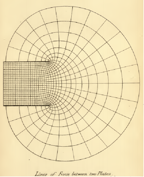
ComplexContourPlot[Im[Log[Sinh[(z/2)]]], {z, -2π , 2π + π I}, ContourShading -> True, AspectRatio -> Automatic, Contours -> 19]ジェームズ クラーク マクスウェル(James Clerk Maxwell)による1873年の「電気磁気論」(A Treatise on Electricity and Magnetism)から,コンデンサを形成する2つの半無限平面の等電位面を示す有名な図 (Fig. XII)を再構築する:
f[z_] := z + E^zInverseFunction[f][z]top = ComplexContourPlot[ReIm[z - ProductLog[1, E^z]], {z, -3π + π I, 2π + 3 π I}]上部の等高線とマッチするように気を付けて,中間部をプロットする:
middle = ComplexContourPlot[ReIm[z - ProductLog[0, E^z]], {z, -3π - π I, 2π + π I}, Contours -> {Range[-10, 2, 0.25], Range[-3, 3, 0.5]}]bottom = ComplexContourPlot[ReIm[z - ProductLog[-1, E^z]], {z, -3π - 3π I, 2π - π I}]Show[top, middle, bottom,
Graphics[{Thick, Red, Line[{{-3π, π}, {-1, π}}],
Line[{{-3π, -π}, {-1, -π}}]}],
PlotRange -> All]その他のアプリケーション (2)
f[z_] := z^5 - 2z^4 + 10z^3 - 2z^2 + 2z - 4{min, {steps}} = Reap[FindRoot[f[z], {z, 2 + I}, StepMonitor :> Sow[z]]];sg = ComplexListPlot[steps, PlotRange -> All, Joined -> True, PlotStyle -> White, Mesh -> All];cg = ComplexContourPlot[Abs[f[z]], {z, -I, 2 + I}];Show[cg, sg]ComplexContourPlot[Evaluate@Table[Abs[z^2 - E^I θ] == 1, {θ, 0, 2π, (π/4)}], {z, 1.5}]特性と関係 (9)
ComplexContourPlotはContourPlotの特殊ケースである:
{ComplexContourPlot[Re[z^2], {z, -2 - 2I, 2 + 2I}],
ContourPlot[Re[(x + I y)^2], {x, -2, 2}, {y, -2, 2}]}ComplexContourPlotは2つ以上の関数の陰影付けを自動的に表示しないようにする:
{ComplexContourPlot[ReIm[z^2], {z, -2 - 2I, 2 + 2I}],
ContourPlot[ReIm[(x + I y)^2], {x, -2, 2}, {y, -2, 2}, ContourShading -> None]}ComplexRegionPlotは複素数上に領域をプロットする:
ComplexRegionPlot[Abs[Log[z]] < 1, {z, 3}]ComplexPlotは色を使って関数の引数と大きさを示す:
ComplexPlot[Log[z], {z, 3}]ComplexPlot3Dを使って
軸を大きさに使う:
ComplexPlot3D[Log[z], {z, 3}]ComplexArrayPlotを複素数の配列に使う:
ComplexArrayPlot[Table[x ^ 3 + I y ^ 2, {x, -2, 2, 0.1}, {y, -2, 2, 0.1}]]ReImPlotとAbsArgPlotを使って複素数値を実数上にプロットする:
ReImPlot[Log[x], {x, -3, 3}]AbsArgPlot[Log[x], {x, -3, 3}]ComplexListPlotを使って複素数の位置を平面上に示す:
ComplexListPlot[RandomComplex[{-3 - 3I, 3 + 3I}, 100]]ComplexStreamPlotとComplexVectorPlotは複素数を方向として扱う:
ComplexStreamPlot[Log[z], {z, 3}]ComplexVectorPlot[Log[z], {z, 3}]考えられる問題 (1)
Arg[f]は
を超えることはないので,ComplexContourPlotは通常は分枝切断線を描画しない:
ComplexContourPlot[Arg[Log[Gamma[z]]] == π, {z, -5 - 5I, 5 + 5I}]関連するガイド
-
▪
- 複素数の可視化
テキスト
Wolfram Research (2020), ComplexContourPlot, Wolfram言語関数, https://reference.wolfram.com/language/ref/ComplexContourPlot.html.
CMS
Wolfram Language. 2020. "ComplexContourPlot." Wolfram Language & System Documentation Center. Wolfram Research. https://reference.wolfram.com/language/ref/ComplexContourPlot.html.
APA
Wolfram Language. (2020). ComplexContourPlot. Wolfram Language & System Documentation Center. Retrieved from https://reference.wolfram.com/language/ref/ComplexContourPlot.html
BibTeX
@misc{reference.wolfram_2026_complexcontourplot, author="Wolfram Research", title="{ComplexContourPlot}", year="2020", howpublished="\url{https://reference.wolfram.com/language/ref/ComplexContourPlot.html}", note=[Accessed: 19-July-2026]}
BibLaTeX
@online{reference.wolfram_2026_complexcontourplot, organization={Wolfram Research}, title={ComplexContourPlot}, year={2020}, url={https://reference.wolfram.com/language/ref/ComplexContourPlot.html}, note=[Accessed: 19-July-2026]}