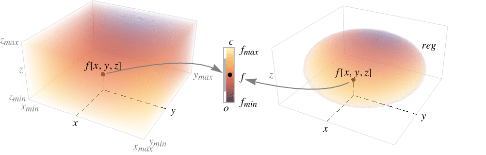
DensityPlot3D[f,{x,xmin,xmax},{y,ymin,ymax},{z,zmin,zmax}]
将 f 作为 x、y 和 z 的函数绘制其密度图线.
DensityPlot3D[f,{x,y,z}∈reg]
在几何区域 reg 内取变量值.
DensityPlot3D
DensityPlot3D[f,{x,xmin,xmax},{y,ymin,ymax},{z,zmin,zmax}]
将 f 作为 x、y 和 z 的函数绘制其密度图线.
DensityPlot3D[f,{x,y,z}∈reg]
在几何区域 reg 内取变量值.
更多信息和选项
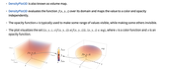
- DensityPlot3D 也被称为体积图.
- DensityPlot3D 在其域上评估函数

,并将其值独立地映射到某个颜色和不透明度. - 不透明度函数
通常用于使某些范围的数值可见,而使其他一些数值不可见. - 该图将
的集合可视化,其中
是一个颜色函数,
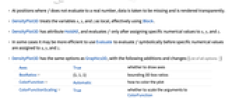
是一个不透明度函数. - 在 f 无法计算得到实数的位置上,数据被认为是缺失的并且渲染成透明的.
- DensityPlot3D 实际上用了 Block 把变量 x、y 和 z 视为局部变量.
- DensityPlot3D 具有属性 HoldAll,并且只有在对 x、y 和 z 赋予特定数值后计算 f.
- 在某些情况下,在对 x、y 和 z 赋予特定数值前使用 Evaluate 符号计算 f 会更高效.
- DensityPlot3D 具有与 Graphics3D 相同的选项,并且有下列添加和变动: [所有选项的列表]
-
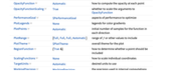
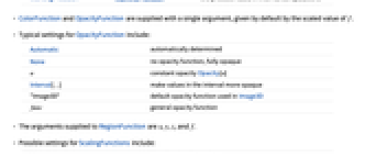
Axes True 是否绘制轴 BoxRatios {1,1,1} 边界三维框比率 ColorFunction Automatic 如何对图线着色 ColorFunctionScaling True 是否缩放 ColorFunction 的参数 OpacityFunction Automatic 如何计算每个点的不透明度 OpacityFunctionScaling True 是否缩放 OpacityFunction 的参数 PerformanceGoal $PerformanceGoal 优化的目标 PlotLegends None 颜色渐变的图例 PlotPoints Automatic 函数在每个方向的样本的初始数目 PlotRange {Full,Full,Full,Automatic} f 的定义域或包含的其他数值 PlotTheme $PlotTheme 绘图的整体主题 RegionFunction (True&) 如何决定是否应该包括一个点 ScalingFunctions None 如何缩放单个坐标 TargetUnits Automatic 使用的预期单位 WorkingPrecision MachinePrecision 用于内部计算的精度 - ColorFunction 和 OpacityFunction 带单个参数,默认由 f 的缩放值给出.
- OpacityFunction 的典型设置包括:
-
Automatic 自动确定 None 无不透明函数,完全不透明 α 常数透明度 Opacity[α] Interval[…] 使区间中的数值更加不透明 "Image3D" Image3D 中使用的默认透明函数 func 普通透明函数 - 对 RegionFunction 提供的参数是 x、y、z 和 f.
- ScalingFunctions 的可能设置包括:
-
sf 缩放 f 等高值 {sx,sy,sz} 缩放 x、y 和 z 轴 {sx,sy,sz,sf} 缩放 x、y 和 z 轴及 f 等高值 - 常见的内置缩放函数 s 包括:
-
"Log" 

带有自动刻度标记的对数刻度 "Log10" 

以 10 为底的对数标尺,刻度为 10 的幂 "SignedLog" 

包含 0 和负数的类对数标尺 "Reverse" 

反转坐标方向 "Infinite" 

无限标尺
所有选项的列表
范例
打开所有单元 关闭所有单元基本范例 (3)
DensityPlot3D[x y z, {x, -1, 1}, {y, -1, 1}, {z, -1, 1}]DensityPlot3D[Sin[x]Cos[y]Sin[z], {x, y, z}∈Ball[{0, 0, 0}, 5], PlotTheme -> "Marketing"]f = PDF[DirichletDistribution[{1, 2, 3, 4}], {x, y, z}]DensityPlot3D[f, {x, 0, 0.5}, {y, 0, 1}, {z, 0, 1}, ColorFunction -> "SunsetColors", PlotLegends -> Automatic]范围 (13)
采样 (6)
DensityPlot3D[Sqrt[x y z], {x, y, z}∈Ball[], OpacityFunction -> None]用 PlotPoints 控制采样:
Table[DensityPlot3D[x y z, {x, -1, 1}, {y, -1, 1}, {z, -1, 1}, PlotPoints -> pp], {pp, {5, 20, 50}}]定义域可以用包括 Cone 在内的区域指定:
DensityPlot3D[x y z, {x, y, z}∈Cone[]]包括 ImplicitRegion 的公式区域:
ℛ = ImplicitRegion[(x ^ 2 + (9 / 4)y ^ 2 + z ^ 2 - 1) ^ 3 - x ^ 2z ^ 3 - (9 / 80)y ^ 2z ^ 3 <= 0, {{x, -1.2, 1.2}, {y, -0.7, 0.7}, {z, -1, 1.3}}];DensityPlot3D[x y z, {x, y, z}∈ℛ]包括 BoundaryMeshRegion 的基于网格的区域:
ℛ = ConvexHullMesh[RandomReal[1, {25, 3}]]DensityPlot3D[x y z, {x, y, z}∈ℛ]使用 PlotRange 限制范围以展示更多详情:
DensityPlot3D[Exp[-(x ^ 2 + y ^ 2 + z ^ 2)], {x, -1, 1}, {y, -1, 1}, {z, -1, 1}, PlotRange -> {{-1, 0}, All, All}, BoxRatios -> Automatic]使用 ClipPlanes 指定一个或者多个剪切平面. 在下面的例子里,剪切
:
DensityPlot3D[Sin[x + y + z] / 10, {x, 0, 10}, {y, 0, 10}, {z, 0, 10}, OpacityFunction -> None, ClipPlanes -> {1, 1, -1, 0}]使用 RegionFunction 更普遍地约束点的包含性:
DensityPlot3D[x ^ 2 + y ^ 2 - z ^ 2, {x, -2, 2}, {y, -2, 2}, {z, -2, 2}, RegionFunction -> Function[{x, y, z, f}, x < y ^ 3]]外观 (7)
使用 PlotTheme 立即获取整体样式:
Table[DensityPlot3D[x y z, {x, -1, 1}, {y, -1, 1}, {z, -1, 1}, PlotLabel -> t, PlotTheme -> t], {t, {"Minimal", "Scientific", "Marketing"}}]用 PlotLegends 获取不同值的颜色条:
DensityPlot3D[x y z, {x, -1, 1}, {y, -1, 1}, {z, -1, 1}, PlotLegends -> Automatic]用 Axes 控制轴的显示:
Table[DensityPlot3D[x y z, {x, -1, 1}, {y, -1, 1}, {z, -1, 1}, PlotLabel -> a, Axes -> a], {a, {True, False, {True, False, True}}}]用 AxesLabel 给轴添加标签,并且使用 PlotLabel 给整个图线添加标签:
DensityPlot3D[x y z, {x, -1, 1}, {y, -1, 1}, {z, -1, 1}, Ticks -> None, AxesLabel -> {x, y, z}, PlotLabel -> x y z]用 ColorFunction 根据函数值对图线着色:
Table[DensityPlot3D[x y z, {x, -1, 1}, {y, -1, 1}, {z, -1, 1}, PlotLabel -> c, ColorFunction -> c], {c, {Hue, "BlueGreenYellow"}}]TargetUnits 指定可视化中使用的单位:
DensityPlot3D[Quantity[x y z, "kg/m^3"], {x, -1, 1}, {y, -1, 1}, {z, -1, 1}, AxesLabel -> Automatic, PlotLegends -> Automatic, TargetUnits -> {"Feet", "Feet", "Feet", "g/ft^3"}]DensityPlot3D[Sin[2π x]Sin[2π y] + z, {x, 0, 1}, {y, 0, 1}, {z, 0, 1}, ScalingFunctions -> {"Log", None, None}]DensityPlot3D[Sin[2π x]Sin[2π y] + z, {x, 0, 1}, {y, 0, 1}, {z, 0, 1}, ScalingFunctions -> {None, None, "Reverse"}]选项 (69)
Axes (4)
默认情况下,DensityPlot3D 会在图中绘制坐标轴:
DensityPlot3D[Sin[2π x]Sin[2π y]Sin[2π z], {x, -1, 1}, {y, -1, 1}, {z, -1, 1}]DensityPlot3D[Sin[2π x]Sin[2π y]Sin[2π z], {x, -1, 1}, {y, -1, 1}, {z, -1, 1}, Axes -> False]用 AxesOrigin 指定坐标轴在何处相交:
DensityPlot3D[Sin[2π x]Sin[2π y]Sin[2π z], {x, -1, 1}, {y, -1, 1}, {z, -1, 1}, AxesOrigin -> {0, 0, 0}]{DensityPlot3D[Sin[2π x]Sin[2π y]Sin[2π z], {x, -1, 1}, {y, -1, 1}, {z, -1, 1}, Axes -> {False, False, True}], DensityPlot3D[Sin[2π x]Sin[2π y]Sin[2π z], {x, -1, 1}, {y, -1, 1}, {z, -1, 1}, Axes -> {True, False, False}], DensityPlot3D[Sin[2π x]Sin[2π y]Sin[2π z], {x, -1, 1}, {y, -1, 1}, {z, -1, 1}, Axes -> {False, True, False}]}AxesLabel (4)
DensityPlot3D[Sin[2π x]Sin[2π y]Sin[2π z], {x, -1, 1}, {y, -1, 1}, {z, -1, 1}]DensityPlot3D[Sin[2π x]Sin[2π y]Sin[2π z], {x, -1, 1}, {y, -1, 1}, {z, -1, 1}, AxesLabel -> z]DensityPlot3D[Sin[2π x]Sin[2π y]Sin[2π z], {x, -1, 1}, {y, -1, 1}, {z, -1, 1}, AxesLabel -> {"X", "Y", "Z"}]用 DensityPlot3D 中指定的变量作为标签:
DensityPlot3D[Sin[2π x]Sin[2π y]Sin[2π z], {x, -1, 1}, {y, -1, 1}, {z, -1, 1}, AxesLabel -> Automatic]AxesOrigin (2)
AxesStyle (4)
DensityPlot3D[Sin[2π x]Sin[2π y]Sin[2π z], {x, -1, 1}, {y, -1, 1}, {z, -1, 1}, AxesStyle -> Red]DensityPlot3D[Sin[2π x]Sin[2π y]Sin[2π z], {x, -1, 1}, {y, -1, 1}, {z, -1, 1}, AxesStyle -> {{Thick, Brown}, {Thick, Blue}, {Thick, Green}}]DensityPlot3D[Sin[2π x]Sin[2π y]Sin[2π z], {x, -1, 1}, {y, -1, 1}, {z, -1, 1}, AxesStyle -> Green, TicksStyle -> StandardBlue]DensityPlot3D[Sin[2π x]Sin[2π y]Sin[2π z], {x, -1, 1}, {y, -1, 1}, {z, -1, 1}, AxesStyle -> Green, LabelStyle -> StandardBlue]BoxRatios (2)
DensityPlot3D[Sin[x ]Cos[y] Sin[z], {x, -Pi / 2, 3Pi / 2}, {y, -Pi / 2, 3Pi / 2}, {z, -3Pi, 3Pi}]使用 BoxRatios->Automatic 显示三维坐标值的自然刻度:
DensityPlot3D[Sin[x ]Cos[y] Sin[z], {x, -Pi / 2, 3Pi / 2}, {y, -Pi / 2, 3Pi / 2}, {z, -3Pi, 3Pi}, BoxRatios -> Automatic]ClipPlanes (3)
使用 ClipPlanes 指定一个或者多个剪切面. 在这个例子里,剪切
:
DensityPlot3D[Sin[x + y + z] / 10, {x, 0, 10}, {y, 0, 10}, {z, 0, 10}, OpacityFunction -> None, ClipPlanes -> {{1, 1, -1, 0}}]DensityPlot3D[Sin[x + y + z] / 10, {x, 0, 10}, {y, 0, 10}, {z, 0, 10}, OpacityFunction -> None, ClipPlanes -> {{1, 1, -1, 0}, {0, 1, 0, -4}}]与普通 RegionFunction 比较:
DensityPlot3D[Sin[x + y + z] / 10, {x, 0, 10}, {y, 0, 10}, {z, 0, 10}, OpacityFunction -> None, RegionFunction -> Function[{x, y, z}, x + y - z ≥ 0]]ColorFunction (1)
ColorFunctionScaling (2)
ColorFunction 的参数通常被缩放为0和1之间的数值:
DensityPlot3D[x + y + z, {x, 0, 3}, {y, 0, 3}, {z, 0, 3}, ColorFunction -> Hue]通过把 ColorFunctionScaling 设置为 False 以使用未缩放密度值:
DensityPlot3D[Sin[2x y z], {x, -2, 2}, {y, -2, 2}, {z, -2, 2}, ColorFunction -> (If[# < 0, Red, Green]&), ColorFunctionScaling -> False, PlotPoints -> 100]ImageSize (7)
使用已命名尺寸,如 Tiny、Small、Medium 和 Large:
{DensityPlot3D[Sin[2π x]Sin[2π y]Sin[2π z], {x, -1, 1}, {y, -1, 1}, {z, -1, 1}, ImageSize -> Tiny], DensityPlot3D[Sin[2π x]Sin[2π y]Sin[2π z], {x, -1, 1}, {y, -1, 1}, {z, -1, 1}, ImageSize -> Small]}{DensityPlot3D[Sin[2π x]Sin[2π y]Sin[2π z], {x, -1, 1}, {y, -1, 1}, {z, -1, 1}, ImageSize -> 150], DensityPlot3D[Sin[2π x]Sin[2π y]Sin[2π z], {x, -1, 1}, {y, -1, 1}, {z, -1, 1}, AspectRatio -> 1.5, ImageSize -> 150]}{DensityPlot3D[Sin[2π x]Sin[2π y]Sin[2π z], {x, -1, 1}, {y, -1, 1}, {z, -1, 1}, ImageSize -> {Automatic, 150}], DensityPlot3D[Sin[2π x]Sin[2π y]Sin[2π z], {x, -1, 1}, {y, -1, 1}, {z, -1, 1}, AspectRatio -> 2, ImageSize -> {Automatic, 150}]}{DensityPlot3D[Sin[2π x]Sin[2π y]Sin[2π z], {x, -1, 1}, {y, -1, 1}, {z, -1, 1}, ImageSize -> UpTo[200]], DensityPlot3D[Sin[2π x]Sin[2π y]Sin[2π z], {x, -1, 1}, {y, -1, 1}, {z, -1, 1}, AspectRatio -> 2, ImageSize -> UpTo[200]]}DensityPlot3D[Sin[2π x]Sin[2π y]Sin[2π z], {x, -1, 1}, {y, -1, 1}, {z, -1, 1}, ImageSize -> {200, 300}, Background -> StandardGray]设置 AspectRatioFull 将填充可用空间:
DensityPlot3D[Sin[2π x]Sin[2π y]Sin[2π z], {x, -1, 1}, {y, -1, 1}, {z, -1, 1}, AspectRatio -> Full, ImageSize -> {200, 300}, Background -> StandardGray]{DensityPlot3D[Sin[2π x]Sin[2π y]Sin[2π z], {x, -1, 1}, {y, -1, 1}, {z, -1, 1}, ImageSize -> {UpTo[150], UpTo[100]}], DensityPlot3D[Sin[2π x]Sin[2π y]Sin[2π z], {x, -1, 1}, {y, -1, 1}, {z, -1, 1}, AspectRatio -> 2, ImageSize -> {UpTo[150], UpTo[100]}]}Framed[Pane[DensityPlot3D[Sin[2π x]Sin[2π y]Sin[2π z], {x, -1, 1}, {y, -1, 1}, {z, -1, 1}, ImageSize -> Full, Background -> StandardGray], {200, 100}]]Framed[Pane[DensityPlot3D[Sin[2π x]Sin[2π y]Sin[2π z], {x, -1, 1}, {y, -1, 1}, {z, -1, 1}, AspectRatio -> Full, ImageSize -> {Scaled[0.5], Scaled[0.5]}, Background -> StandardGray], {200, 200}]]OpacityFunction (6)
默认情况下 OpacityFunction 是 Automatic:
DensityPlot3D[x y z, {x, -1, 1}, {y, -1, 1}, {z, -1, 1}]设置 OpacityFunctionNone 下关闭透明度:
DensityPlot3D[x y z, {x, -1, 1}, {y, -1, 1}, {z, -1, 1}, OpacityFunction -> None]DensityPlot3D[Sin[π x]Sin[π y] Sin[π z], {x, -1, 1}, {y, -1, 1}, {z, -1, 1}, OpacityFunction -> Interval[{-1, -0.6}, {0.6, 1}], OpacityFunctionScaling -> False, PlotLegends -> Automatic]使用常量透明度 Opacity[0.05]:
DensityPlot3D[Sin[π x]Sin[π y] Sin[π z], {x, -1, 1}, {y, -1, 1}, {z, -1, 1}, OpacityFunction -> 0.05, PlotLegends -> Automatic]使用与 Image3D 中相同的不透明度函数:
f = PDF[DirichletDistribution[{1, 2, 3, 4}], {x, y, z}];DensityPlot3D[f, {x, 0, 1}, {y, 0, 1}, {z, 0, 1}, OpacityFunction -> "Image3D", PlotLegends -> Automatic]DensityPlot3D[x y z, {x, -1, 1}, {y, -1, 1}, {z, -1, 1}, OpacityFunction -> Function[f, (1 - f) ^ 2]]OpacityFunctionScaling (3)
DensityPlot3D[x y z, {x, -1, 1}, {y, -1, 1}, {z, -1, 1}, OpacityFunction -> Function[f, (1 - f) ^ 2]]通过把 OpacityFunctionScaling 设置为 False,使用未缩放的密度值:
DensityPlot3D[x + y + z, {x, -1, 1}, {y, -1, 1}, {z, -1, 1}, OpacityFunction -> Function[f, If[f > 0, 1, 0]], OpacityFunctionScaling -> False]DensityPlot3D[x y z, {x, -1, 1}, {y, -1, 1}, {z, -1, 1}, OpacityFunction -> Interval[{-1, 0}], OpacityFunctionScaling -> False, PlotLegends -> Automatic, ColorFunction -> "BrightBands"]PerformanceGoal (2)
PlotLegends (2)
DensityPlot3D[x y z, {x, -1, 1}, {y, -1, 1}, {z, -1, 1}]使用 PlotLegends->Automatic 显示图例图线:
DensityPlot3D[x y z, {x, -1, 1}, {y, -1, 1}, {z, -1, 1}, PlotLegends -> Automatic]PlotPoints (2)
PlotRange (3)
DensityPlot3D[Exp[-(x ^ 2 + y ^ 2 + z ^ 2)], {x, -1, 1}, {y, -1, 1}, {z, -1, 1}]DensityPlot3D[Exp[-(x ^ 2 + y ^ 2 + z ^ 2)], {x, -1, 1}, {y, -1, 1}, {z, -1, 1}, PlotRange -> {{-1, 0}, All, All}, BoxRatios -> Automatic]DensityPlot3D[x ^ 2 + y ^ 2 - z ^ 2, {x, -2, 2}, {y, -2, 2}, {z, -2, 2}, PlotRange -> {0, 1}]DensityPlot3D[x ^ 2 + y ^ 2 - z ^ 2, {x, -2, 2}, {y, -2, 2}, {z, -2, 2}, PlotRange -> {All, All, All, {0, 1}}]PlotTheme (3)
DensityPlot3D[x y z, {x, -1, 1}, {y, -1, 1}, {z, -1, 1}, PlotTheme -> "Marketing"]DensityPlot3D[x y z, {x, -1, 1}, {y, -1, 1}, {z, -1, 1}, PlotTheme -> "Marketing", FaceGrids -> None]Table[DensityPlot3D[x y z, {x, -1, 1}, {y, -1, 1}, {z, -1, 1}, PlotLabel -> t, PlotTheme -> t, ImageSize -> 130], {t, {"Scientific", "Monochrome", "Minimal", "Web", "Working", "Classic", "Business", "Marketing", "Detailed"}}]RegionFunction (3)
DensityPlot3D[x ^ 2 + y ^ 2 - z ^ 2, {x, -2, 2}, {y, -2, 2}, {z, -2, 2}, RegionFunction -> Function[{x, y, z, f}, x ^ 2 + y ^ 2 + z ^ 2 ≤ 4]]DensityPlot3D[x ^ 2 + y ^ 2 - z ^ 2, {x, -2, 2}, {y, -2, 2}, {z, -2, 2}, RegionFunction -> Function[{x, y, z, f}, f < 2]]DensityPlot3D[x ^ 2 + y ^ 2 - z ^ 2, {x, -2, 2}, {y, -2, 2}, {z, -2, 2}, RegionFunction -> Function[{x, y, z, f}, x < -1 || x > 1]]ScalingFunctions (4)
默认情况下,DensityPlot3D 在所有方向都有线性标尺:
DensityPlot3D[x + y + z, {x, 0, 10}, {y, 0, 10}, {z, 0, 10}]DensityPlot3D[x + y + z, {x, 0, 10}, {y, 0, 10}, {z, 0, 10}, ScalingFunctions -> {"Log", None, None}]使用 ScalingFunctions 在
方向反转坐标方向:
DensityPlot3D[x + y + z, {x, 0, 10}, {y, 0, 10}, {z, 0, 10}, ScalingFunctions -> {None, None, "Reverse"}]DensityPlot3D[x + y + z, {x, 0, 10}, {y, 0, 10}, {z, 0, 10}, ScalingFunctions -> {{-Log[#]&, Exp[-#]&}, None, None}]TargetUnits (2)
轴和图例按照由 TargetUnits 指定的单位添加标签:
DensityPlot3D[x y z, {x, -1, 1}, {y, -1, 1}, {z, -1, 1}, AxesLabel -> Automatic, PlotLegends -> Automatic, TargetUnits -> {"Meters", "Meters", "Meters", "kg/m^3"}]由 Quantity 指定的单位转化为由 TargetUnits 指定的单位:
DensityPlot3D[Quantity[x y z, "kg/m^3"], {x, -1, 1}, {y, -1, 1}, {z, -1, 1}, PlotLegends -> Automatic, TargetUnits -> "g/ft^3"]Ticks (6)
DensityPlot3D[ Cos[ y] Sin[z], {x, -2, 2}, {y, -2, 2}, {z, -2, 2}]DensityPlot3D[ Cos[ y] Sin[z], {x, -2, 2}, {y, -2, 2}, {z, -2, 2}, Ticks -> None]DensityPlot3D[ Cos[ y] Sin[z], {x, -2, 2}, {y, -2, 2}, {z, -2, 2}, Ticks -> {{-1.5, 0, 1.5}, {-1.5, 0, 1.5}, {-1.5, 0, 1.5}}]DensityPlot3D[ Cos[ y] Sin[z], {x, -2, 2}, {y, -2, 2}, {z, -2, 2}, Ticks -> {{{-1.5, -a}, {0, 0}, {1.5, a}}, {{-1.5, -a}, {0, 0}, {1.5, a}}, {{-1.5, -a}, {0, 0}, {1.5, a}}}]DensityPlot3D[ Cos[ y] Sin[z], {x, -2, 2}, {y, -2, 2}, {z, -2, 2}, Ticks -> {{{-1.5, -a, .1}, {0, 0, .1}, {1.5, a, .1}}, {{-1.5, -a, .05}, {0, 0, .05}, {1.5, a, .05}}, {{-1.5, -a, .15}, {0, 0, .15}, {1.5, a, .15}}}]DensityPlot3D[ Cos[ y] Sin[z], {x, -2, 2}, {y, -2, 2}, {z, -2, 2}, Ticks -> {{{-1.5, -a, .1, Directive[Red, Dashed, Thick]}, {0, 0, .1, Directive[Red, Dashed]}, {1.5, a, .1, Directive[Red]}}, {{-1.5, -a, .05, Directive[Blue, Dashed, Thick]}, {0, 0, .05, Directive[Blue, Dashed]}, {1.5, a, .05, Directive[Blue]}}, {{-1.5, -a, .15, Directive[Darker@Green, Dashed, Thick]}, {0, 0, .15, Directive[Darker@Green, Dashed]}, {1.5, a, .15, Directive[Darker@Green]}}}]TicksStyle (3)
DensityPlot3D[ Cos[ y] Sin[z], {x, -2, 2}, {y, -2, 2}, {z, -2, 2}, AxesStyle -> Directive[Thick, Red]]DensityPlot3D[ Cos[ y] Sin[z], {x, -2, 2}, {y, -2, 2}, {z, -2, 2}, TicksStyle -> Directive[Bold, Red]]DensityPlot3D[ Cos[ y] Sin[z], {x, -2, 2}, {y, -2, 2}, {z, -2, 2}, TicksStyle -> {Directive[Green, Bold], Directive[Bold, Red], Directive[Bold, Blue]}]应用 (17)
Elementary Functions (4)
DensityPlot3D[x, {x, -2, 2}, {y, -2, 2}, {z, -2, 2}]{DensityPlot3D[y, {x, -2, 2}, {y, -2, 2}, {z, -2, 2}],
DensityPlot3D[z, {x, -2, 2}, {y, -2, 2}, {z, -2, 2}]}{DensityPlot3D[x + y, {x, -2, 2}, {y, -2, 2}, {z, -2, 2}],
DensityPlot3D[y + z, {x, -2, 2}, {y, -2, 2}, {z, -2, 2}]}{DensityPlot3D[x + y + z, {x, -2, 2}, {y, -2, 2}, {z, -2, 2}],
DensityPlot3D[x - y + z, {x, -2, 2}, {y, -2, 2}, {z, -2, 2}]}{DensityPlot3D[x ^ 2 + y ^ 2, {x, -2, 2}, {y, -2, 2}, {z, -2, 2}], DensityPlot3D[y ^ 2 + z ^ 2, {x, -2, 2}, {y, -2, 2}, {z, -2, 2}]}{DensityPlot3D[x ^ 2 + y ^ 2 + z ^ 2, {x, -2, 2}, {y, -2, 2}, {z, -2, 2}], DensityPlot3D[x ^ 2 + y ^ 2 + 2z ^ 2, {x, -2, 2}, {y, -2, 2}, {z, -2, 2}]}DensityPlot3D[Sin[π x]Sin[π y]Sin[π z], {x, -2, 2}, {y, -2, 2}, {z, -2, 2}]{DensityPlot3D[Sin[π x]Sin[π (y + z)], {x, -2, 2}, {y, -2, 2}, {z, -2, 2}], DensityPlot3D[Sin[π (x + y)]Sin[π z], {x, -2, 2}, {y, -2, 2}, {z, -2, 2}]}DensityPlot3D[Sin[π (x + y + z)], {x, -2, 2}, {y, -2, 2}, {z, -2, 2}]f = Exp[-Norm[{x, y, z} - {-1, -1, -1}]^2] + Exp[-Norm[{x, y, z} - {1, 1, 1}]^2];DensityPlot3D[f, {x, -2, 2}, {y, -2, 2}, {z, -2, 2}]f = Sum[Exp[-2Norm[{x, y, z} - pi]^2], {pi, RandomPoint[Cuboid[{-1, -1, -1}, {1, 1, 1}], 10]}];DensityPlot3D[f, {x, -2, 2}, {y, -2, 2}, {z, -2, 2}]Distribution Functions (6)
绘制分布的 PDF 图线:
𝒟 = MultinormalDistribution[{0, 0, 0}, {{1, 0.5, 0}, {0.5, 1, 0}, {0, 0, 1}}];
f = PDF[𝒟, {x, y, z}];d = DensityPlot3D[f, {x, -2, 2}, {y, -2, 2}, {z, -2, 2}]pts = RandomVariate[𝒟, 10 ^ 4];Show[d, Graphics3D[{Green, AbsolutePointSize[1], Point[pts]}]]绘制分布的 CDF 图线:
𝒟 = MultinormalDistribution[{0, 0, 0}, {{1, 0.5, 0}, {0.5, 1, 0}, {0, 0, 1}}];
cdf = CDF[𝒟, {x, y, z}];DensityPlot3D[cdf, {x, -2, 2}, {y, -2, 2}, {z, -2, 2}, PlotLegends -> Automatic]sf = SurvivalFunction[𝒟, {x, y, z}];DensityPlot3D[sf, {x, -2, 2}, {y, -2, 2}, {z, -2, 2}, PlotLegends -> Automatic]hf = HazardFunction[𝒟, {x, y, z}];DensityPlot3D[hf, {x, -2, 2}, {y, -2, 2}, {z, -2, 2}, PlotLegends -> Automatic]探索 MultinormalDistribution 的 Correlation 参数,其中 ρab 是 a 和 b 之间的相关性:
cov[{σx_, σy_, σz_}, {ρxy_, ρyz_, ρxz_}] := {{σx^2, σx σy ρxy, σx σz ρxz}, {σx σy ρxy, σy^2, σy σz ρyz}, {σx σz ρxz, σy σz ρyz, σz^2}};Σ = cov[{1, 1, 1}, {0.5, 0, 0}];
f = PDF[MultinormalDistribution[{0, 0, 0}, Σ], {x, y, z}];DensityPlot3D[f, {x, -2, 2}, {y, -2, 2}, {z, -2, 2}]Σ = cov[{1, 1, 1}, {0, 0.5, 0}];
f = PDF[MultinormalDistribution[{0, 0, 0}, Σ], {x, y, z}];DensityPlot3D[f, {x, -2, 2}, {y, -2, 2}, {z, -2, 2}]只有 y 和 z 之间的相关性,但是 z 分量中较大的方差
:
Σ = cov[{1, 1, 2}, {0, 0.5, 0}];
f = PDF[MultinormalDistribution[{0, 0, 0}, Σ], {x, y, z}];DensityPlot3D[f, {x, -2, 2}, {y, -2, 2}, {z, -4, 4}, BoxRatios -> Automatic]可视化 ProductDistribution 的 PDF:
𝒟 = ProductDistribution[{NormalDistribution[0, 1], 3}];
f = PDF[𝒟, {x, y, z}]DensityPlot3D[f, {x, -2, 2}, {y, -2, 2}, {z, -2, 2}]𝒟 = ProductDistribution[NormalDistribution[], LaplaceDistribution[], WeibullDistribution[1, 1]];
f = PDF[𝒟, {x, y, z}]DensityPlot3D[f, {x, -2, 2}, {y, -2, 2}, {z, 0, 5}]𝒟 = ProductDistribution[BinormalDistribution[1 / 2], ExponentialDistribution[3]];
f = PDF[𝒟, {x, y, z}]DensityPlot3D[f, {x, -2, 2}, {y, -2, 2}, {z, 0, 3}]绘制 CopulaDistribution 的 PDF:
𝒟 = CopulaDistribution[{"Frank", 1}, {GammaDistribution[3, 2 / 3], ExponentialDistribution[2], NormalDistribution[]}];
f = PDF[𝒟, {x, y, z}]DensityPlot3D[f, {x, 0, 6}, {y, 0, 3}, {z, -3, 3}]可视化一些三变量数据的内核密度估计的 PDF:
data = RandomVariate[NormalDistribution[], {1000, 3}];
f = PDF[SmoothKernelDistribution[data], {x, y, z}];DensityPlot3D[f, {x, -3, 3}, {y, -3, 3}, {z, -3, 3}]使用 ClipPlanes 查看内部:
DensityPlot3D[f, {x, -3, 3}, {y, -3, 3}, {z, -3, 3}, ClipPlanes -> {1, 1, -1, 0}]Partial Differential Equations (3)
在周期性边界条件下可视化非线性正弦-Gordon 方程,其中时间用
轴表示:
L = 4;
usol = NDSolveValue[{D[u[t, x, y], t, t] == D[u[t, x, y], x, x] + D[u[t, x, y], y, y] + Sin[u[t, x, y]], u[t, -L, y] == u[t, L, y], u[t, x, -L] == u[t, x, L], u[0, x, y] == Exp[-(x ^ 2 + y ^ 2)], Derivative[1, 0, 0][u][0, x, y] == 0}, u, {t, 0, L / 2}, {x, -L, L}, {y, -L, L}]DensityPlot3D[usol[t, x, y], {x, -L, L}, {y, -L, L}, {t, 0, L / 2}, AxesLabel -> Automatic, PlotLegends -> Automatic]DensityPlot3D[usol[t, x, y], {x, -L, L}, {y, -L, L}, {t, 0, L / 2}, AxesLabel -> Automatic, ClipPlanes -> {0, 1, 0, 0}]在两个空间维度内可视化 Wolfram 非线性波动方程,其中时间在
轴上表示:
usol = NDSolveValue[{D[u[t, x, y], t, t] == D[u[t, x, y], x, x] + D[u[t, x, y], y, y] / 2 + (1 - u[t, x, y] ^ 2)(1 + 2u[t, x, y]), u[0, x, y] == E^-(x^2 + y^2), u[t, -5, y] == u[t, 5, y], u[t, x, -5] == u[t, x, 5], u^(1, 0, 0)[0, x, y] == 0}, u, {t, 0, 4}, {x, -5, 5}, {y, -5, 5}]DensityPlot3D[usol[t, x, y], {x, -5, 5}, {y, -5, 5}, {t, 1, 4}, AxesLabel -> Automatic, ClipPlanes -> {0, 1, 0, 0}, ColorFunction -> "BrightBands", PlotLegends -> Automatic]可视化三维偏微分方程的解. 在这个例子里,是 Ball 上的具有狄利克雷边界条件的泊松方程:

usol = NDSolveValue[{Subsuperscript[∇, {x, y, z}, 2]u[x, y, z] == 1, DirichletCondition[u[x, y, z] == x y z, True]}, u, {x, y, z}∈Ball[]]DensityPlot3D[usol[x, y, z], {x, y, z}∈Ball[], PlotLegends -> Automatic]Potential and Wave Functions (4)
v = Total[Table[1 / Norm[{x, y, z} - p], {p, RandomReal[{-0.5, 0.5}, {5, 3}]}]];DensityPlot3D[v, {x, -1, 1}, {y, -1, 1}, {z, -1, 1}]f = Sum[Cos[10 Norm[{x, y, z} - {Sin[θ], 0, Cos[θ]}]], {θ, 0, (4 π/3), (2 π/3)}]DensityPlot3D[f, {x, -1, 1}, {y, -1, 1}, {z, -1, 1}, PlotTheme -> "Minimal"]f = (((x y) Exp[I ((6π/5) - π Sqrt[x^2 + y^2 + z^2])]) (-1 + 2 I + (3 + I/Sqrt[x^2 + y^2 + z^2]))/(x^2 + y^2 + z^2) Sqrt[x^2 + y^2 + z^2]);DensityPlot3D[Clip[Re[f], {-50, 50}], {x, -0.5, 0.5}, {y, -0.5, 0.5}, {z, -0.5, 0.5}, PlotLegends -> Automatic, OpacityFunctionScaling -> False, OpacityFunction -> Interval[{-50, -10}, {10, 50}], ColorFunction -> "RedGreenSplit"]a0 = Quantity["BohrRadius"] / Quantity["Meters"]ψ[{n_, l_, m_}, {r_, θ_, ϕ_}] := With[{ρ = 2r / (n a0)}, Sqrt[((2/n a0))^3((n - l - 1)!/2n(n + l)!)]Exp[-ρ / 2]ρ^lLaguerreL[n - l - 1, 2l + 1, ρ]SphericalHarmonicY[l, m, θ, ϕ]]DensityPlot3D[(Abs@ψ[{2, 1, 0}, {Sqrt[x^2 + y^2 + z^2], ArcTan[z, Sqrt[x^2 + y^2]], ArcTan[x, y]}])^2, {x, -5 a0, 5 a0}, {y, -5 a0, 5 a0}, {z, -5 a0, 5 a0}, PlotLegends -> Automatic]属性和关系 (5)
对于数据,使用 ListDensityPlot3D:
data = Table[x y z, {x, -1, 1, 0.05}, {y, -1, 1, 0.05}, {z, -1, 1, 0.05}];{ListDensityPlot3D[data], DensityPlot3D[x y z, {x, -2, 2}, {y, -2, 2}, {z, -2, 2}]}对于二维空间中的密度图线,使用 DensityPlot:
{DensityPlot[x ^ 2 + y ^ 2, {x, -1, 1}, {y, -1, 1}], DensityPlot3D[x ^ 2 + y ^ 2, {x, -1, 1}, {y, -1, 1}, {z, -1, 1}, OpacityFunction -> None]}对于切片曲面上的密度图线,使用 SliceDensityPlot3D:
{SliceDensityPlot3D[x y z, "BackPlanes", {x, -2, 2}, {y, -2, 2}, {z, -2, 2}], DensityPlot3D[x y z, {x, -2, 2}, {y, -2, 2}, {z, -2, 2}]}对于切片曲面上的等高线使用 SliceContourPlot3D:
{SliceContourPlot3D[x y z, "BackPlanes", {x, -2, 2}, {y, -2, 2}, {z, -2, 2}], DensityPlot3D[x y z, {x, -2, 2}, {y, -2, 2}, {z, -2, 2}]}对常量值曲面使用 ContourPlot3D:
{ContourPlot3D[x ^ 2 + y ^ 2 + z ^ 2, {x, -2, 2}, {y, -2, 2}, {z, -2, 2}], DensityPlot3D[x ^ 2 + y ^ 2 + z ^ 2, {x, -2, 2}, {y, -2, 2}, {z, -2, 2}]}文本
Wolfram Research (2015),DensityPlot3D,Wolfram 语言函数,https://reference.wolfram.com/language/ref/DensityPlot3D.html (更新于 2022 年).
CMS
Wolfram 语言. 2015. "DensityPlot3D." Wolfram 语言与系统参考资料中心. Wolfram Research. 最新版本 2022. https://reference.wolfram.com/language/ref/DensityPlot3D.html.
APA
Wolfram 语言. (2015). DensityPlot3D. Wolfram 语言与系统参考资料中心. 追溯自 https://reference.wolfram.com/language/ref/DensityPlot3D.html 年
BibTeX
@misc{reference.wolfram_2026_densityplot3d, author="Wolfram Research", title="{DensityPlot3D}", year="2022", howpublished="\url{https://reference.wolfram.com/language/ref/DensityPlot3D.html}", note=[Accessed: 08-September-2026]}
BibLaTeX
@online{reference.wolfram_2026_densityplot3d, organization={Wolfram Research}, title={DensityPlot3D}, year={2022}, url={https://reference.wolfram.com/language/ref/DensityPlot3D.html}, note=[Accessed: 08-September-2026]}