


StreamPlot3D
StreamPlot3D[{vx,vy,vz},{x,xmin,xmax},{y,ymin,ymax},{z,zmin,zmax}]
绘制作为 x、y 和 z 的函数的向量场 {vx,vy,vz} 的流线.
StreamPlot3D[{vx,vy,vz},{x,y,z}∈reg]
将变量 {x,y,z} 视为位于几何区域 reg 中.
更多信息和选项
- StreamPlot3D 被称为三维流图或流线图. 除了线,流线还可以显示为管(流管)和带(流带).
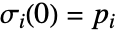
- StreamPlot3D 绘制由
 和
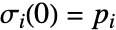 定义的流线
 ,其中
 和
 是初始流点. 流线
 是通过点
 的曲线,其切线对应于各点处的矢量场
 .
- 流线默认根据矢量场
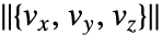 的大小
 着色.
- StreamPlot3D 缺省情况下显示足够多的流线,从而使得整个图形的密度大致均匀,且不显示背景标量场.
- StreamPlot3D 将变量 x、y 和 z 视为局部变量,实际上相当于使用 Block.
- StreamPlot3D 具有属性 HoldAll,仅在指定 x、y 和 z 的数值后才计算 vi 等等. 有些情况下,先用 Evaluate 符号式计算 vi 等会更有效.
- StreamPlot3D 有和 Graphics 相同的选项,不同之处及更多选项如下所示: [所有选项的列表]
-
BoxRatios {1,1,1} 高宽比 EvaluationMonitor None 每次运行函数时要计算的表达式 Method Automatic 绘图时使用的方法 PerformanceGoal $PerformanceGoal 优化的目标 PlotLegends None 包含的图例 PlotRange {Full,Full,Full} 包含的 x、y、z 值的范围 PlotRangePadding Automatic 对数值范围进行多少填充 PlotTheme $PlotTheme 绘图的整体外观主题 RegionBoundaryStyle Automatic 怎样设置绘图区域边界的样式 RegionFunction True& 确定要包含的区域 ScalingFunctions None 怎样缩放个别坐标 StreamColorFunction Automatic 如何为流线着色 StreamColorFunctionScaling True 是否缩放传递给 StreamColorFunction 的参数 StreamMarkers Automatic 流的形状 StreamPoints Automatic 流线的数量和流线的放置 StreamScale None 如何缩放流线的大小 StreamStyle Automatic 如何绘制流线 WorkingPrecision MachinePrecision 内部计算使用的精度 - 提供给 RegionFunction 和 StreamColorFunction 中的函数的参数为 x,y,z,vx,vy,vz,Norm[{vx,vy,vz}].
- StreamMarkers 的可能的设置包括:
-

"Arrow" 带有 2D 箭头的线段 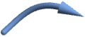
"Arrow3D" 带有 3D 箭头的管状线段 
"Line" 线段 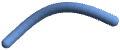
"Tube" 管状线段 
"Ribbon" 扁平丝带 
"ArrowRibbon" 带有内置箭头的丝带 - 如果设置 StreamScaleAutomatic 并使用 "arrow" 流线标记,流线将被分割为多个线段,以便于查看流线的方向.
- StreamScale 的可能的设置包括:
-
Automatic 自动确定流线的线段 Full 将流线显示为一个整体 Tiny,Small,Medium,Large 表明线段长度的已命名设置 {len,npts,ratio} 使用明确的流线线段指定 - 流线线段的长度 len 可为以下形式之一:
-
Automatic 自动确定长度 None 将流线显示为一个整体 Tiny,Small,Medium,Large 使用已命名的线段长度 s 使用与图形大小的比例为 s 的长度 - 用来画出每个线段的点数 npts 可以是 Automatic 或特定的点数.
- 比值 ratio 指定流线的截面相对于线段的宽度.
- ScalingFunctions 的可能设置包括:
-
{sx,sy,sz} 缩放 x、y 和 z 坐标 - 常见的内置缩放函数 s 包括:
-
"Log" 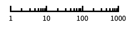
对数刻度,自动进行标记 "Log10" 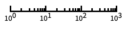
以 10 为底的对数刻度,用 10 的幂进行标记 "SignedLog" 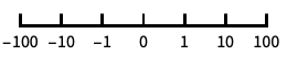
类似对数的刻度,包含 0 和负数 "Reverse" 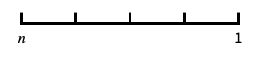
反转坐标的方向 "Infinite" 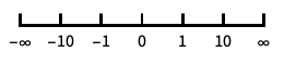
无穷刻度
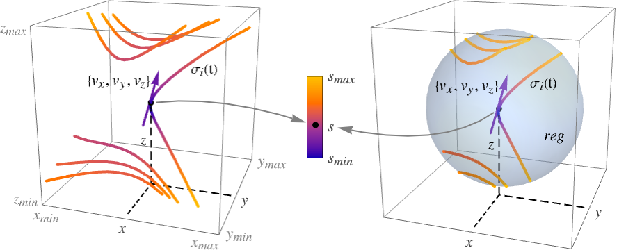
所有选项的列表
范例
打开所有单元 关闭所有单元基本范例 (4)
StreamPlot3D[{x, y, 1}, {x, -1, 1}, {y, -1, 1}, {z, -1, 1}]StreamPlot3D[{y^2, 1, x}, {x, -1, 1}, {y, -1, 1}, {z, -1, 1}, StreamMarkers -> "Tube"]StreamPlot3D[{1, y, ArcTan[x]}, {x, -1, 1}, {y, -1, 1}, {z, -1, 1}, PlotLegends -> Automatic]StreamPlot3D[{z, -x, y}, {x, y, z}∈Ball[]]范围 (12)
采样 (3)
StreamPlot3D[{x, y, 1}, {x, -1, 1}, {y, -1, 1}, {z, -1, 1}, StreamPoints -> Coarse]StreamPlot3D[{x, y, 1}, {x, -1, 1}, {y, -1, 1}, {z, -1, 1}, StreamPoints -> RandomReal[{-1, 1}, {30, 3}]]StreamPlot3D[{x, y, 1}, {x, -1, 1}, {y, -1, 1}, {z, -1, 1}, RegionFunction -> Function[{x, y, z}, x^2 + y^2 ≤ 1]]演示 (9)
StreamPlot3D[{y, -x, y - x}, {x, -1, 1}, {y, -1, 1}, {z, -1, 1}]StreamPlot3D[{y, -x, y - x}, {x, -1, 1}, {y, -1, 1}, {z, -1, 1}, StreamMarkers -> "Tube"]StreamPlot3D[{y, -x, y - x}, {x, -1, 1}, {y, -1, 1}, {z, -1, 1}, StreamMarkers -> "Ribbon"]StreamPlot3D[{z, -x, y + x}, {x, -1, 1}, {y, -1, 1}, {z, -1, 1}, StreamMarkers -> "Arrow"]StreamPlot3D[{z, -x, y + x}, {x, -1, 1}, {y, -1, 1}, {z, -1, 1}, StreamMarkers -> "Arrow3D"]StreamPlot3D[{z, -x, y + x}, {x, -1, 1}, {y, -1, 1}, {z, -1, 1}, StreamMarkers -> "ArrowRibbon"]StreamPlot3D[{y, -x, y - x}, {x, -1, 1}, {y, -1, 1}, {z, -1, 1}, StreamColorFunction -> None]StreamPlot3D[{y, -x, y - x}, {x, -1, 1}, {y, -1, 1}, {z, -1, 1}, StreamColorFunction -> "DarkRainbow"]StreamPlot3D[{y, -x, y - x}, {x, -1, 1}, {y, -1, 1}, {z, -1, 1}, PlotLegends -> Automatic]用 StreamScale 把流线分成多个较短的线段:
StreamPlot3D[{x, y, 1}, {x, -1, 1}, {y, -1, 1}, {z, -1, 1}, StreamScale -> 0.1]StreamPlot3D[{x, y, 1}, {x, -1, 1}, {y, -1, 1}, {z, -1, 1}, StreamScale -> 0.2]StreamPlot3D[{x, y, 1}, {x, -1, 1}, {y, -1, 1}, {z, -1, 1}, StreamMarkers -> "Arrow", StreamScale -> {Full, 20, 0.2}]StreamPlot3D[{x, y, 1}, {x, -1, 1}, {y, -1, 1}, {z, -1, 1}, PlotTheme -> "Marketing"]StreamPlot3D[{x, y, z}, {x, 1, 100}, {y, 1, 100}, {z, 1, 100}, ScalingFunctions -> {"Log", None, None}]StreamPlot3D[{x, y, z}, {x, 1, 100}, {y, 1, 100}, {z, 1, 100}, ScalingFunctions -> {None, None, "Reverse"}]选项 (70)
Axes (3)
默认情况下,绘制 Axes:
StreamPlot3D[{y - z, z - x, x - y}, {x, -2, 2}, {y, -1, 1}, {z, -1, 1}]StreamPlot3D[{y - z, z - x, x - y}, {x, -2, 2}, {y, -1, 1}, {z, -1, 1}, Axes -> False]{StreamPlot3D[{y - z, z - x, x - y}, {x, -2, 2}, {y, -1, 1}, {z, -1, 1}, Axes -> {True, False, False}], StreamPlot3D[{y - z, z - x, x - y}, {x, -2, 2}, {y, -1, 1}, {z, -1, 1}, Axes -> {False, True, False}], StreamPlot3D[{y - z, z - x, x - y}, {x, -2, 2}, {y, -1, 1}, {z, -1, 1}, Axes -> {False, False, True}]}AxesLabel (3)
StreamPlot3D[{y - z, z - x, x - y}, {x, -2, 2}, {y, -1, 1}, {z, -1, 1}]
StreamPlot3D[{y - z, z - x, x - y}, {x, -2, 2}, {y, -1, 1}, {z, -1, 1}, AxesLabel -> z]StreamPlot3D[{y - z, z - x, x - y}, {x, -2, 2}, {y, -1, 1}, {z, -1, 1}, AxesLabel -> {x, y, z}]AxesOrigin (2)
AxesStyle (4)
StreamPlot3D[{y - z, z - x, x - y}, {x, -2, 2}, {y, -1, 1}, {z, -1, 1}, AxesStyle -> StandardRed]StreamPlot3D[{y - z, z - x, x - y}, {x, -2, 2}, {y, -1, 1}, {z, -1, 1}, AxesStyle -> {{Thick, StandardBrown}, {Thick, StandardBlue}, {Thick, StandardGreen}}]StreamPlot3D[{y - z, z - x, x - y}, {x, -2, 2}, {y, -1, 1}, {z, -1, 1}, AxesStyle -> StandardGreen, TicksStyle -> StandardGray]StreamPlot3D[{y - z, z - x, x - y}, {x, -2, 2}, {y, -1, 1}, {z, -1, 1}, AxesStyle -> StandardGreen, LabelStyle -> StandardGray]BoxRatios (2)
ImageSize (7)
使用已命名尺寸,如 Tiny、Small、Medium 和 Large:
{StreamPlot3D[{y, -x, y - x}, {x, -1, 1}, {y, -1, 1}, {z, -1, 1}, ImageSize -> Tiny], StreamPlot3D[{y, -x, y - x}, {x, -1, 1}, {y, -1, 1}, {z, -1, 1}, ImageSize -> Small]}{StreamPlot3D[{y, -x, y - x}, {x, -1, 1}, {y, -1, 1}, {z, -1, 1}, ImageSize -> 150], StreamPlot3D[{y, -x, y - x}, {x, -1, 1}, {y, -1, 1}, {z, -1, 1}, AspectRatio -> 1.5, ImageSize -> 150]}{StreamPlot3D[{y, -x, y - x}, {x, -1, 1}, {y, -1, 1}, {z, -1, 1}, ImageSize -> {Automatic, 150}], StreamPlot3D[{y, -x, y - x}, {x, -1, 1}, {y, -1, 1}, {z, -1, 1}, AspectRatio -> 2, ImageSize -> {Automatic, 150}]}{StreamPlot3D[{y, -x, y - x}, {x, -1, 1}, {y, -1, 1}, {z, -1, 1}, ImageSize -> UpTo[200]], StreamPlot3D[{y, -x, y - x}, {x, -1, 1}, {y, -1, 1}, {z, -1, 1}, AspectRatio -> 2, ImageSize -> UpTo[200]]}StreamPlot3D[{y, -x, y - x}, {x, -1, 1}, {y, -1, 1}, {z, -1, 1}, ImageSize -> {200, 300}, Background -> StandardBlue]设置 AspectRatioFull 将填充可用空间:
StreamPlot3D[{y, -x, y - x}, {x, -1, 1}, {y, -1, 1}, {z, -1, 1}, AspectRatio -> Full, ImageSize -> {200, 300}, Background -> StandardBlue]{StreamPlot3D[{y, -x, y - x}, {x, -1, 1}, {y, -1, 1}, {z, -1, 1}, ImageSize -> {UpTo[150], UpTo[100]}], StreamPlot3D[{y, -x, y - x}, {x, -1, 1}, {y, -1, 1}, {z, -1, 1}, AspectRatio -> 2, ImageSize -> {UpTo[150], UpTo[100]}]}Framed[Pane[StreamPlot3D[{y, -x, y - x}, {x, -1, 1}, {y, -1, 1}, {z, -1, 1}, ImageSize -> Full, Background -> StandardBlue], {200, 200}]]Framed[Pane[StreamPlot3D[{y, -x, y - x}, {x, -1, 1}, {y, -1, 1}, {z, -1, 1}, AspectRatio -> Full, ImageSize -> {Scaled[0.5], Scaled[0.5]}, Background -> StandardBlue], {200, 200}]]PlotLegends (3)
StreamPlot3D[{y z, x z, x y}, {x, -1, 1}, {y, -1, 1}, {z, -1, 1}]StreamPlot3D[{y z, x z, x y}, {x, -1, 1}, {y, -1, 1}, {z, -1, 1}, PlotLegends -> Automatic]StreamPlot3D[{y z, x z, x y}, {x, -1, 1}, {y, -1, 1}, {z, -1, 1}, PlotLegends -> Placed[Automatic, Left]]PlotTheme (1)
RegionBoundaryStyle (4)
显示 RegionFunction 定义的区域:
StreamPlot3D[{-4 x^2 y - 4 y^3 - x z, 4 x^3 + 4 x y^2 - y z, x^2 + y^2}, {x, -1, 1}, {y, -1, 1}, {z, -1, 1}, RegionFunction -> (#1^2 + #2^2 + #3^2 < 1&)]用 None 不显示边界:
StreamPlot3D[{-4 x^2 y - 4 y^3 - x z, 4 x^3 + 4 x y^2 - y z, x^2 + y^2}, {x, -1, 1}, {y, -1, 1}, {z, -1, 1}, RegionFunction -> (#1^2 + #2^2 + #3^2 < 1&), RegionBoundaryStyle -> None]StreamPlot3D[{-4 x^2 y - 4 y^3 - x z, 4 x^3 + 4 x y^2 - y z, x^2 + y^2}, {x, -1, 1}, {y, -1, 1}, {z, -1, 1}, RegionFunction -> (#1^2 + #2^2 + #3^2 < 1&), RegionBoundaryStyle -> Orange]StreamPlot3D[{-4 x^2 y - 4 y^3 - x z, 4 x^3 + 4 x y^2 - y z, x^2 + y^2}, {x, -1, 1}, {y, -1, 1}, {z, -1, 1}]RegionFunction (4)
StreamPlot3D[{-4 x^2 y - 4 y^3 - x z, 4 x^3 + 4 x y^2 - y z, x^2 + y^2}, {x, -1, 1}, {y, -1, 1}, {z, -1, 1}, RegionFunction -> (#1^2 + #2^2 + #3^2 < 1&)]StreamPlot3D[{-4 x^2 y - 4 y^3 - x z, 4 x^3 + 4 x y^2 - y z, x^2 + y^2}, {x, -1, 1}, {y, -1, 1}, {z, -1, 1}, RegionFunction -> (#7 > 2&)]StreamPlot3D[{x, y, 1}, {x, -2, 2}, {y, -2, 2}, {z, -2, 2}, RegionFunction -> Function[{x, y, z, vx, vy, vz, n}, vx vy > 0]]用 RegionBoundaryStyleNone 不显示边界:
StreamPlot3D[{-4 x^2 y - 4 y^3 - x z, 4 x^3 + 4 x y^2 - y z, x^2 + y^2}, {x, -1, 1}, {y, -1, 1}, {z, -1, 1}, RegionFunction -> (#1^2 + #2^2 + #3^2 < 1&), RegionBoundaryStyle -> None]ScalingFunctions (1)
StreamColorFunction (4)
StreamPlot3D[{x, 2y, 3z}, {x, -1, 1}, {y, -1, 1}, {z, -1, 1}, StreamColorFunction -> Hue]使用来自 ColorData 的已命名颜色梯度:
StreamPlot3D[{x, 2y, 3z}, {x, -1, 1}, {y, -1, 1}, {z, -1, 1}, StreamColorFunction -> "Rainbow"]StreamPlot3D[{x, 2y, 3z}, {x, -1, 1}, {y, -1, 1}, {z, -1, 1}, StreamColorFunction -> Function[{x, y, z, vx, vy, vz, n}, Hue[x]]]用 StreamColorFunctionScalingFalse 获取未缩放的值:
StreamPlot3D[{x, 2y, 3z}, {x, -1, 1}, {y, -1, 1}, {z, -1, 1}, StreamColorFunction -> "Rainbow", StreamColorFunctionScaling -> False]StreamColorFunctionScaling (2)
StreamPlot3D[{y, -x, 10z}, {x, -1, 1}, {y, -1, 1}, {z, -1, 1}, StreamColorFunction -> "Pastel", PlotLegends -> Automatic]用 StreamColorFunctionScalingFalse 获取未缩放的值:
StreamPlot3D[{y, -x, 10z}, {x, -1, 1}, {y, -1, 1}, {z, -1, 1}, StreamColorFunction -> "BlueGreenYellow", PlotLegends -> Automatic, StreamColorFunctionScaling -> False]StreamMarkers (5)
StreamPlot3D[{-4 x^2 y - 4 y^3 - x z, 4 x^3 + 4 x y^2 - y z, x^2 + y^2}, {x, -1, 1}, {y, -1, 1}, {z, -1, 1}]StreamPlot3D[IconizedObject[«field»], IconizedObject[«vars»], StreamMarkers -> "Tube"]StreamPlot3D[IconizedObject[«field»], IconizedObject[«vars»], StreamMarkers -> "Ribbon"]带有 "Arrow" 的流线标记会自动将流线断开成更短的线段:
StreamPlot3D[IconizedObject[«field»], IconizedObject[«vars»], StreamMarkers -> "Arrow"]StreamPlot3D[IconizedObject[«field»], IconizedObject[«vars»], StreamMarkers -> "Arrow3D"]StreamPlot3D[IconizedObject[«field»], IconizedObject[«vars»], StreamMarkers -> "ArrowRibbon"]StreamPlot3D[{x, y, 1}, {x, -1, 1}, {y, -1, 1}, {z, -1, 1}, StreamMarkers -> "Arrow3D", StreamScale -> Full]StreamPlot3D[{x, y, 1}, {x, -1, 1}, {y, -1, 1}, {z, -1, 1}, StreamMarkers -> "Ribbon", StreamScale -> 0.1]StreamPoints (4)
StreamPlot3D[{y^2, 1, x}, {x, -1, 1}, {y, -1, 1}, {z, -1, 1}]StreamPlot3D[{y^2, 1, x}, {x, -1, 1}, {y, -1, 1}, {z, -1, 1}, StreamPoints -> 25]StreamPlot3D[{y^2, 1, x}, {x, -1, 1}, {y, -1, 1}, {z, -1, 1}, StreamPoints -> RandomReal[{-1, 1}, {20, 3}]]StreamPlot3D[{y^2, 1, x}, {x, -1, 1}, {y, -1, 1}, {z, -1, 1}, StreamPoints -> Coarse]StreamPlot3D[{y^2, 1, x}, {x, -1, 1}, {y, -1, 1}, {z, -1, 1}, StreamPoints -> Fine]StreamScale (9)
StreamPlot3D[{1, y, ArcTan[x]}, {x, -1, 1}, {y, -1, 1}, {z, -1, 1}, StreamMarkers -> "Arrow"]StreamPlot3D[{1, y, ArcTan[x]}, {x, -1, 1}, {y, -1, 1}, {z, -1, 1}, StreamMarkers -> "Arrow", StreamScale -> 0.2]StreamPlot3D[{1, y, ArcTan[x]}, {x, -1, 1}, {y, -1, 1}, {z, -1, 1}, StreamMarkers -> "Arrow", StreamScale -> {0.2, 2}]StreamPlot3D[{1, y, ArcTan[x]}, {x, -1, 1}, {y, -1, 1}, {z, -1, 1}, StreamMarkers -> "Arrow", StreamScale -> {0.2, 2, 0.2}]StreamPlot3D[{1, y, ArcTan[x]}, {x, -1, 1}, {y, -1, 1}, {z, -1, 1}, StreamMarkers -> "Arrow", StreamScale -> Full]StreamPlot3D[{1, y, ArcTan[x]}, {x, -1, 1}, {y, -1, 1}, {z, -1, 1}, StreamMarkers -> "Ribbon", StreamScale -> 0.2]{StreamPlot3D[{1, y, ArcTan[x]}, {x, -1, 1}, {y, -1, 1}, {z, -1, 1}, StreamMarkers -> "Ribbon", StreamScale -> {Automatic, Automatic, 0.05}], StreamPlot3D[{1, y, ArcTan[x]}, {x, -1, 1}, {y, -1, 1}, {z, -1, 1}, StreamMarkers -> "Tube", StreamScale -> {Automatic, Automatic, 0.05}]}{StreamPlot3D[{1, y, ArcTan[x]}, {x, -1, 1}, {y, -1, 1}, {z, -1, 1}, StreamMarkers -> "Ribbon", StreamScale -> {Automatic, Automatic, 0.1}], StreamPlot3D[{1, y, ArcTan[x]}, {x, -1, 1}, {y, -1, 1}, {z, -1, 1}, StreamMarkers -> "Tube", StreamScale -> {Automatic, Automatic, 0.1}]}{StreamPlot3D[{1, y, ArcTan[x]}, {x, -1, 1}, {y, -1, 1}, {z, -1, 1}, StreamMarkers -> "Arrow", StreamScale -> {Automatic, Automatic, 0.15}], StreamPlot3D[{1, y, ArcTan[x]}, {x, -1, 1}, {y, -1, 1}, {z, -1, 1}, StreamMarkers -> "Arrow", StreamScale -> {Automatic, Automatic, 0.2}]}{StreamPlot3D[{-4 x^2 y - 4 y^3 - x z, 4 x^3 + 4 x y^2 - y z, x^2 + y^2}, {x, -1, 1}, {y, -1, 1}, {z, -1, 1}, StreamScale -> {0.5, 5}, ...], StreamPlot3D[{-4 x^2 y - 4 y^3 - x z, 4 x^3 + 4 x y^2 - y z, x^2 + y^2}, {x, -1, 1}, {y, -1, 1}, {z, -1, 1}, StreamScale -> {0.5, 20}, ...]}StreamStyle (3)
StreamPlot3D[{x, y, 1}, {x, -1, 1}, {y, -1, 1}, {z, -1, 1}, StreamStyle -> Thickness[0.02]]StreamColorFunction 的优先级比 StreamStyle 高:
StreamPlot3D[{x, y, 1}, {x, -1, 1}, {y, -1, 1}, {z, -1, 1}, StreamStyle -> Directive[Red, Dashing[{0.1, 0.01}]]]设置 StreamColorFunctionNone,通过 StreamStyle 指定流线的颜色:
StreamPlot3D[{x, y, 1}, {x, -1, 1}, {y, -1, 1}, {z, -1, 1}, StreamStyle -> Directive[StandardRed, Dashing[{0.1, 0.01}]], StreamColorFunction -> None]Ticks (6)
StreamPlot3D[{x, y, 1 / y}, {x, -2, 2}, {y, -2, 2}, {z, -2, 2}]StreamPlot3D[{x, y, 1 / y}, {x, -2, 2}, {y, -2, 2}, {z, -2, 2}, Ticks -> None]StreamPlot3D[{x, y, 1 / y}, {x, -2, 2}, {y, -2, 2}, {z, -2, 2}, Ticks -> {{-1.5, 0, 1.5}, {-1.5, 0, 1.5}, {-1.5, 0, 1.5}}]StreamPlot3D[{x, y, 1 / y}, {x, -2, 2}, {y, -2, 2}, {z, -2, 2}, Ticks -> {{{-1.5, -a}, {0, 0}, {1.5, a}}, {{-1.5, -a}, {0, 0}, {1.5, a}}, {{-1.5, -a}, {0, 0}, {1.5, a}}}]StreamPlot3D[{x, y, 1 / y}, {x, -2, 2}, {y, -2, 2}, {z, -2, 2}, Ticks -> {{{-1.5, -a, .1}, {0, 0, .1}, {1.5, a, .1}}, {{-1.5, -a, .05}, {0, 0, .05}, {1.5, a, .05}}, {{-1.5, -a, .15}, {0, 0, .15}, {1.5, a, .15}}}]StreamPlot3D[{x, y, 1 / y}, {x, -2, 2}, {y, -2, 2}, {z, -2, 2}, Ticks -> {{{-1.5, -a, .1, Directive[Red, Dashed, Thick]}, {0, 0, .1, Directive[Red, Dashed]}, {1.5, a, .1, Directive[Red]}}, {{-1.5, -a, .05, Directive[StandardGray, Dashed, Thick]}, {0, 0, .05, Directive[StandardGray, Dashed]}, {1.5, a, .05, Directive[StandardGray]}}, {{-1.5, -a, .15, Directive[Darker@Green, Dashed, Thick]}, {0, 0, .15, Directive[Darker@Green, Dashed]}, {1.5, a, .15, Directive[Darker@Green]}}}]TicksStyle (3)
StreamPlot3D[{x, y, 1 / y}, {x, -2, 2}, {y, -2, 2}, {z, -2, 2}, AxesStyle -> Directive[Bold, StandardRed]]StreamPlot3D[{x, y, 1 / y}, {x, -2, 2}, {y, -2, 2}, {z, -2, 2}, TicksStyle -> Directive[Bold, StandardRed]]StreamPlot3D[{x, y, 1 / y}, {x, -2, 2}, {y, -2, 2}, {z, -2, 2}, TicksStyle -> {Directive[StandardGray, Bold], Directive[Bold, StandardRed], Directive[Bold, StandardBlue]}]应用 (10)
基本应用 (1)


流体的流动 (3)
来考虑形为 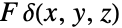 的点力的 Stokes 流,其中
 是常向量,
 是 Dirac delta 函数. 例如,向下的力:
F = {0, 0, -1};


vars = {x, y, z};
μ = 1;
u = (1/8π μ)Table[Sum[( (vars[[i]]vars[[j]]/(vars.vars)^3 / 2) + (IdentityMatrix[3][[i, j]]/Sqrt[vars.vars]))F[[j]], {j, 1, 3}], {i, 1, 3}];
p = (1/4π)Sum[(vars[[j]]F[[j]]/(vars.vars)^3 / 2), {j, 1, 3}];

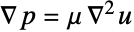
{Div[u, vars] == 0, Grad[p, vars] == μ Laplacian[u, vars]}//SimplifyStreamPlot3D[u, {x, -3, 3}, {y, -3, 3}, {z, -3, 3}, StreamMarkers -> "Arrow3D", PlotLegends -> Automatic]可视化单位球体周围的 Stokes 流. 定义流体的速度向量  、压力
 、粘度
 和远场流体速度
 :
vars = {x, y, z};
μ = 1;
U = 1;
u = {U, 0, 0} - (3/4)(x (U vars/(vars.vars)^3 / 2) + ({U, 0, 0}/Sqrt[vars.vars])) - (1/4)(({U, 0, 0}/(vars.vars)^3 / 2) - (3U x vars/(vars.vars)^5 / 2));
p = -(3μ x/2(vars.vars)^3 / 2);
{Div[u, vars] == 0, Grad[p, vars] == μ Laplacian[u, vars]}//SimplifyShow[StreamPlot3D[u, {x, -4, 4}, {y, -2, 2}, {z, -2, 2}, PlotLegends -> Automatic, StreamMarkers -> "Arrow", StreamPoints -> Flatten[Table[{-3, y, z}, {y, -1.75, 1.75, 0.5}, {z, -1.75, 1.75, 0.5}], 1]], Graphics3D[{Yellow, Sphere[]}], BoxRatios -> {2, 1, 1}]DensityPlot3D[p, {x, -4, 4}, {y, -2, 2}, {z, -2, 2}, PlotLegends -> Automatic, RegionFunction -> Function[{x, y, z}, x^2 + y^2 + z^2 > 1], BoxRatios -> {2, 1, 1}]指定流体流过有一个凸起的管道的Navier–Stokes 方程:
velocities = {u[x, y, z], v[x, y, z], w[x, y, z]};
navierstokes = {
    Inactive[
       Div][(-μ Inactive[Grad][u[x, y, z], {x, y, z}]), {x, y,
       z}] + ρ  *
      velocities.Inactive[Grad][u[x, y, z], {x, y, z}] +
p^(1, 0, 0)[x, y, z],
    Inactive[
       Div][(-μ Inactive[Grad][v[x, y, z], {x, y, z}]), {x, y,
       z}] + ρ  *
      velocities.Inactive[Grad][v[x, y, z], {x, y, z}] +
p^(0, 1, 0)[x, y, z],
    Inactive[
       Div][(-μ Inactive[Grad][w[x, y, z], {x, y, z}]), {x, y,
       z}] + ρ  *
      velocities.Inactive[Grad][w[x, y, z], {x, y, z}] +
p^(0, 0, 1)[x, y, z],

u^(1, 0, 0)[x, y, z] + v^(0, 1, 0)[x, y, z] + w^(0, 0, 1)[x, y, z]} /. {μ -> 10 ^ -3, ρ -> 1};Ω = RegionUnion[Ball[], Cylinder[{{-2, 0, 0}, {2, 0, 0}}, 1 / 2]];
RegionPlot3D[Ω]inflowBC = DirichletCondition[{u[x, y, z] == 0.2, v[x, y, z] == 0, w[x, y, z] == 0}, x == -2];
outflowBC = DirichletCondition[p[x, y, z] == 0, x == 2];
wallBC = DirichletCondition[{u[x, y, z] == 0, v[x, y, z] == 0, w[x, y, z] == 0}, -2 < x < 2];
bcs = {inflowBC, outflowBC, wallBC};{uVel, vVel, wVel, pressure} = NDSolveValue[{navierstokes == {0, 0, 0, 0}, bcs}, {u, v, w, p}, {x, y, z}∈Ω, Method -> {"FiniteElement", "InterpolationOrder" -> {u -> 2, v -> 2, w -> 2, p -> 1}, "MeshOptions" -> {"MaxCellMeasure" -> 0.01}}];sp = Prepend[#, 0]& /@ Flatten[Table[CirclePoints[r, 10], {r, {0.3, 0.5, 0.7, 0.9}}], 1];StreamPlot3D[{uVel[x, y, z], vVel[x, y, z], wVel[x, y, z]}, {x, -2, 2}, {y, -1, 1}, {z, -1, 1}, RegionFunction -> Function[{x, y, z}, {x, y, z}∈Ω], StreamPoints -> sp, BoxRatios -> {2, 1, 1}, Method -> {"IntegrationLimits" -> 100}, StreamMarkers -> "Arrow", StreamScale -> {0.05, Automatic, 0.07}, ImageSize -> Medium]电子系统 (1)
StreamPlot3D[({x, y, z - 1}/Norm[{x, y, z - 1}]^3) - ({x, y, z + 1}/Norm[{x, y, z + 1}]^3), {x, -3, 3}, {y, -3, 3}, {z, -3, 3}]由于向量场的范数在  处的点电荷附近的变化异常快速,因此流线的颜色似乎都一样. 将向量场范数的幅值与区域函数绑定在一起即可显示出不同的颜色:
StreamPlot3D[({x, y, z - 1}/Norm[{x, y, z - 1}]^3) - ({x, y, z + 1}/Norm[{x, y, z + 1}]^3), {x, -3, 3}, {y, -3, 3}, {z, -3, 3}, RegionFunction -> (#7 < 5&), RegionBoundaryStyle -> None, PlotLegends -> Automatic]Show[StreamPlot3D[({x, y, z - 1}/Norm[{x, y, z - 1}]^3) - ({x, y, z + 1}/Norm[{x, y, z + 1}]^3), {x, -3, 3}, {y, -3, 3}, {z, -3, 3}, RegionFunction -> (#7 < 5&), RegionBoundaryStyle -> None, PlotLegends -> Automatic], Graphics3D[{Red, Sphere[{0, 0, 1}, 0.2], Black, Sphere[{0, 0, -1}, 0.2]}]]可添加箭头来提供更多信息,但是颜色会发生变化,因为箭头标记是根据箭头尖端处的场强度来着色的:
Show[StreamPlot3D[({x, y, z - 1}/Norm[{x, y, z - 1}]^3) - ({x, y, z + 1}/Norm[{x, y, z + 1}]^3), {x, -3, 3}, {y, -3, 3}, {z, -3, 3}, RegionFunction -> (#7 < 5&), RegionBoundaryStyle -> None, PlotLegends -> Automatic, StreamMarkers -> "Arrow3D"], Graphics3D[{StandardRed, Sphere[{0, 0, 1}, 0.2], StandardGray, Sphere[{0, 0, -1}, 0.2]}]]使用自定义的 StreamColorFunction 对颜色施加更多控制:
Show[StreamPlot3D[({x, y, z - 1}/Norm[{x, y, z - 1}]^3) - ({x, y, z + 1}/Norm[{x, y, z + 1}]^3), {x, -3, 3}, {y, -3, 3}, {z, -3, 3}, RegionFunction -> (0.01 < #7 < 5&), RegionBoundaryStyle -> None, StreamColorFunction -> (Blend[{GrayLevel[0], GrayLevel[1], RGBColor[1, 0, 0]}, #3]&), StreamMarkers -> "Arrow"], Graphics3D[{StandardRed, Sphere[{0, 0, 1}, 0.2], StandardGray, Sphere[{0, 0, -1}, 0.2]}]]其他 (5)
StreamPlot3D[{10(y - x), x(28 - z) - y, x y - (8/3) z}, {x, -30, 30}, {y, -30, 30}, {z, 0, 50}, StreamPoints -> {{1, 1, 1}}]StreamPlot3D[{1, 2x, 3x^2}, {x, -1, 1}, {y, -1, 1}, {z, -1, 1}, StreamMarkers -> "ArrowRibbon", StreamPoints -> {{0, 0, 0}}, ViewPoint -> {-1.3, 2.4, 2}]StreamPlot3D[{-y, x, x^2 - y^2}, {x, -2, 2}, {y, -2, 2}, {z, -2, 2}, StreamPoints -> Table[{r, 0, 0}, {r, 0, 2, 0.2}]]可视化 Poiseuille 流的流线. 中心轴上的流体速度最快:
StreamPlot3D[{1 - y^2 - z^2, 0, 0}, {x, -2, 2}, {y, -1, 1}, {z, -1, 1}, BoxRatios -> {2, 1, 1}, PlotLegends -> Automatic, RegionFunction -> Function[{x, y, z}, y^2 + z^2 ≤ 1], StreamMarkers -> "Arrow", StreamPoints -> Flatten[Table[Prepend[#, 0]& /@ CirclePoints[r, 10], {r, 0.1, 1, 0.1}], 1]]moments = {1, 2, 3};
StreamPlot3D[Evaluate[(| | | |
| --- | --- | --- |
| 0 | -x3 | x2 |
| x3 | 0 | -x1 |
| -x2 | x1 | 0 |).({x1, x2, x3}/moments)], {x1, -1, 1}, {x2, -1, 1}, {x3, -1, 1}, StreamPoints -> SpherePoints[40]]属性和关系 (9)
通过 VectorPlot3D 用离散的箭头可视化场:
VectorPlot3D[{z, -x, y}, {x, -2, 2}, {y, -2, 2}, {z, -2, 2}]用 ListStreamPlot3D 或 ListVectorPlot3D 根据数据绘图:
data = Table[{z, -x, y}, {x, -2, 2}, {y, -2, 2}, {z, -2, 2}];{ListStreamPlot3D[data], ListVectorPlot3D[data]}用 StreamPlot 绘制二维向量场的流线:
StreamPlot[{-1 - x ^ 2 + y, 1 + x - y ^ 2}, {x, -3, 3}, {y, -3, 3}]通过 VectorPlot 用向量而不是流线绘图:
VectorPlot[{-1 - x ^ 2 + y, 1 + x - y ^ 2}, {x, -3, 3}, {y, -3, 3}]data = Table[{-1 - x ^ 2 + y, 1 + x - y ^ 2}, {x, -3, 3, 0.1}, {y, -3, 3, 0.1}];{ListStreamPlot[data], ListVectorPlot[data]}使用 StreamDensityPlot 添加标量场的密度图:
StreamDensityPlot[{-1 - x ^ 2 + y, 1 + x - y ^ 2}, {x, -3, 3}, {y, -3, 3}]通过 VectorDensityPlot 用箭头而不是流线绘图:
VectorDensityPlot[{-1 - x ^ 2 + y, 1 + x - y ^ 2}, {x, -3, 3}, {y, -3, 3}]data = Table[{-1 - x ^ 2 + y, 1 + x - y ^ 2}, {x, -3, 3, 0.1}, {y, -3, 3, 0.1}];{ListStreamDensityPlot[data], ListVectorDensityPlot[data]}用 LineIntegralConvolutionPlot 绘制向量场的线积分卷积:
LineIntegralConvolutionPlot[{-1 - x ^ 2 + y, 1 + x - y ^ 2}, {x, -3, 3}, {y, -3, 3}]使用 VectorDisplacementPlot 可视化与位移矢量场相关的区域的变形:
VectorDisplacementPlot[{y, x - x^3}, {x, y}∈Disk[], VectorPoints -> Automatic]使用 ListVectorDisplacementPlot 根据数据可视化相同的变形:
data = Table[{{x, y} = RandomReal[{-1, 1}, {2}], {y, x - x ^ 3}}, {300}];ListVectorDisplacementPlot[data, Disk[], VectorPoints -> Automatic]用 SliceVectorPlot3D 沿曲面绘制向量:
SliceVectorPlot3D[{x, y, z}, "CenterPlanes", {x, -1, 1}, {y, -1, 1}, {z, -1, 1}]data = Table[{x, y, z}, {x, -1, 1}, {y, -1, 1}, {z, -1, 1}];ListSliceVectorPlot3D[data, "CenterPlanes"]使用 VectorDisplacementPlot3D 可视化与位移矢量场相关的三维区域的变形:
VectorDisplacementPlot3D[{y, x, -z}, {x, 0, 1}, {y, 0, 1}, {z, 0, 1}, VectorPoints -> "Boundary"]使用 ListVectorDisplacementPlot3D 根据数据可视化相同的变形:
data = Table[{{x, y, z} = RandomReal[{0, 1}, {3}], {y, x, -z}}, {300}];ListVectorDisplacementPlot3D[data, Cuboid[], VectorPoints -> "Boundary"]使用 ComplexVectorPlot 或 ComplexStreamPlot 将复变量的复函数可视化为向量场或流线:
{ComplexVectorPlot[Sin[3z], {z, 2}], ComplexStreamPlot[Sin[3z], {z, 2}]}用 GeoVectorPlot 在地图上绘制矢量:
GeoVectorPlot[GeoVector[GeoPosition[{{-54.79801473961214, -111.85053058521567},
    {-65.56940402358214, 162.89657500795147}, {-81.67990688759895, -93.36222177594851},
    {7.785750774919734, 95.44840765141487}, {-6.86571958448036, -40.946398330539864},
    { ... 904, "AngularDegrees"]},
   {0.9366099079317551, Quantity[357.70482317743733, "AngularDegrees"]},
   {0.8256817194791912, Quantity[242.07227508889662, "AngularDegrees"]},
   {0.2661401145642981, Quantity[152.90003252279325, "AngularDegrees"]}}]]
使用 GeoStreamPlot 绘制流线而不是矢量:
GeoStreamPlot[GeoVector[GeoPosition[{{-54.79801473961214, -111.85053058521567},
    {-65.56940402358214, 162.89657500795147}, {-81.67990688759895, -93.36222177594851},
    {7.785750774919734, 95.44840765141487}, {-6.86571958448036, -40.946398330539864},
    { ... 904, "AngularDegrees"]},
   {0.9366099079317551, Quantity[357.70482317743733, "AngularDegrees"]},
   {0.8256817194791912, Quantity[242.07227508889662, "AngularDegrees"]},
   {0.2661401145642981, Quantity[152.90003252279325, "AngularDegrees"]}}]]
可能存在的问题 (3)
管状 StreamMarkers 可能被 BoxRatios 扭曲:
StreamPlot3D[{2, -10 z - x y, 10 y - x z}, {x, -2π, 2π}, {y, -1, 1}, {z, -1, 1}, StreamMarkers -> "Tube"]仔细调整 BoxRatios 可消除失真现象:
StreamPlot3D[{2, -10 z - x y, 10 y - x z}, {x, -2π, 2π}, {y, -1, 1}, {z, -1, 1}, StreamMarkers -> "Tube", BoxRatios -> {2π, 1, 1}]"Arrow" 和 "Arrow3D" 流线标记的颜色由箭头的尖端确定,这可能导致长箭头的颜色不一致:
StreamPlot3D[{ArcTan[z], y, -x}, {x, -5, 5}, {y, -5, 5}, {z, -5, 5}]StreamPlot3D[{ArcTan[z], y, -x}, {x, -5, 5}, {y, -5, 5}, {z, -5, 5}, StreamMarkers -> "Arrow3D", StreamScale -> Full]文本
Wolfram Research (2021),StreamPlot3D,Wolfram 语言函数,https://reference.wolfram.com/language/ref/StreamPlot3D.html (更新于 2022 年).
CMS
Wolfram 语言. 2021. "StreamPlot3D." Wolfram 语言与系统参考资料中心. Wolfram Research. 最新版本 2022. https://reference.wolfram.com/language/ref/StreamPlot3D.html.
APA
Wolfram 语言. (2021). StreamPlot3D. Wolfram 语言与系统参考资料中心. 追溯自 https://reference.wolfram.com/language/ref/StreamPlot3D.html 年