



TimeSeries
TimeSeries[{{t1,v1},{t2,v2},…,{tn,vn}}]
時点と値のペア{ti,vi}で指定された時系列を表す.
TimeSeries[tvspec]
時点と値の指定 tvspec を使う.
TimeSeries[vspec,tspec]
tspec で指定された時点の値 vspec を持つ時系列を表す.
TimeSeries[vspec,tspec,{com1,com2,…}]
一意的な時系列成分のキー com1, com2, …を指定する.
詳細とオプション
- TimeSeriesは,対応する成分値を伴う一連のタイムスタンプを表す.データ点の間にも常に何らかの値が存在すると仮定される.
- 時系列は,通常,徐々に変化する何らかの対象を表現するために用いられるもので,データ点の間における値がどのようなものであり得るかについては,さまざまなモデルが存在する.
- 典型的な時系列の用途:
-
自然 温度,気圧,風速等 社会 株価,インフレーション,失業率,GDP等 技術 エネルギー生産,速度,電圧等 医療 体温,心拍数,血糖値,ECG等 - TimeSeriesオブジェクト ts の時点 t における値は,ts[t]を用いて計算される.
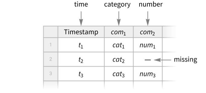
- TimeSeriesオブジェクトは,常に,キー列としての"Timestamp"と任意個の成分値列を持つTabularオブジェクトとして見ることができる.Tabular[TimeSeries[…]]はTabularオブジェクトに変換される.
- TimeSeriesは,事象を数えること,値を累積すること,または局所的な事象率を計算することによって,EventSeriesから導出することが可能であり,そのような変換を提供するのがEventSeriesAccumulateである.
- EventSeriesは,ゼロ交差,最大値交差,その他の事象等の事象を検出することでTimeSeriesから導出でき,TimeSeriesEventsはそのような変換を提供する.
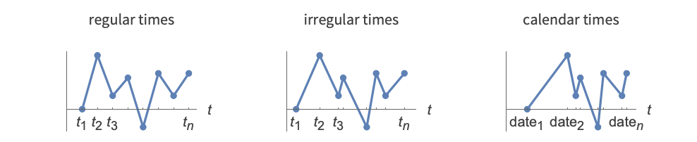
- 時点 ti は規則的な場合も不規則な場合もあり,数値である場合もあればDateObjectのインスタンスである場合もある.
- 以下の時間と値の指定 tvspec を与えることができる:
-
{{t1,v1},{t2,v2},…,{tn,vn}}, 時点と値のペアの集合 timesvalues 時点と値を個別に指定する Tabular[…] Tabularオブジェクト - 時点と値のペアの集合は入力時に順序付けられている必要はないが,出力時には自動的に順序付けられ,パスを形成する.
- 以下の時点指定 tspec を与えることができる:
-
Automatic  ,
 個の値に対する
{tmin} 
{tmin,tmax}  ,自動的に決定される
 に対する
{tmin,Automatic,dt} 
{{t1,t2,…,tn}} 時刻のリスト 
{TabularColumn[…]} 時点のTabularColumn - ti,tminおよび tmaxは,数値またはDateObjectのインスタンスとすることができる.dt は,数値,時間的なQuantity,または日付型("BusinessDay","Weekday","Weekend","BeginningOfMonth","EndOfMonth",あるいはMondayからSundayまで)とすることができる.
- 以下の値指定 vspec を与えることができる:
-
{v1,v2,…,vn} 値のリスト Tabular[…], TabularColumn[…] 値のTabularまたはTabularColumn - 時間系列または事象系列 tes について,TimeSeries[tes,options]は,指定されたオプションを持つTimeSeriesオブジェクトを返す.
- TimeSeriesオブジェクト ts の特性は,ts["property"]から取得できる.
- 利用可能な特性のリストは,ts["Properties"]を用いて取得できる.
- 利用可能なタイムスタンプの特性には次のものが含まれる:
-
"Timestamps" タイムスタンプのTabularColumn "FirstTimestamp" 最初のタイムスタンプ "LastTimestamp" 最後のタイムスタンプ "Dates" DateObjectのリストとしてのタイムスタンプ "Times" AbsoluteTimeのリストとしてのタイムスタンプ "FirstDate", "FirstTime" DateObjectまたはAbsoluteTimeとしての最初のタイムスタンプ "LastDate", "LastTime" DateObjectまたはAbsoluteTimeとしての最後のタイムスタンプ - 利用可能な値の特性には以下が含まれる:
-
"Values" TabularオブジェクトまたはTabularColumnオブジェクトとしての値 "NormalValues" リスト{v1,…}としての値 "FirstValue" 最初のタイムスタンプにおける値 v1 "LastValue" 最後のタイムスタンプにおける値 "ValueType" 単純な時系列の値の型 "ComponentKeys" パス成分のキー "ComponentTypes" パス成分の型 - 利用可能な一般的な特性には次のものが含まれる:
-
"Tabular" 時系列をTabularオブジェクトに変換する "ResamplingMethod" パス成分をリサンプリングするために使用する方法 "NormalPath" 順序付けられたタイムスタンプと値のペア{{t1,v1},…} "Path" AbsoluteTimeとしてのタイムスタンプを持つパス "DatePath" DateObjectとしてのタイムスタンプを持つパス "PathLength" パスの長さ "PathComponents" 多変量経路を一変量成分に分割する "PathFunction" 時間の関数としてのもとの時系列 - Normal[ts] は ts["NormalPath"]と等価である.
- TimeSeriesは次のオプションを取る.
-
ComponentKeys Automatic パス構成要素のキー CalendarType Automatic 使用する暦の種類 DateGranularity Automatic 暦のタイムスタンプの粒度 HolidayCalendar Automatic 使用する休日暦 TimeSystem Automatic 使用する時間系 TimeZone Automatic 使用する時刻帯 DateFunction Automatic 日付を標準形式に変換する方法 MergingFunction Automatic 重複するタイムスタンプの値を統合する方法 MetaInformation None 追加のメタ情報を含めるかどうか MissingDataMethod None 欠損値に使用する方法 ResamplingMethod Automatic リサンプリングに使用する方法 InterpolationOrder Automatic リサンプリングに使用する補間次数 TemporalRegularity Automatic データを規則的であると仮定するかどうか TimeObservationWindow Automatic タイムスタンプの時間領域を指定する ValueDimensions Automatic 値の次元 - デフォルトでは,リサンプリングにはゼロ次または一次の補間が使用され,同一次元の値に対しては一次が使用され,それ以外のすべての場合にはゼロ次が用いられる. opts は Interpolationに渡されるオプションであるときには設定 ResamplingMethod->{"Interpolation",opts}が指定できる.
- MissingDataMethod->Automaticと設定すると,ResamplingMethodの設定に従った補間を用いて,頭部がMissingである値が自動的に置き換えられる.
- 設定ValueDimensions->dim は,値 vijの次元が dim であるように指定する.



例題
すべて開く すべて閉じる例 (2)
ts = TimeSeries[{23.1, 24.4, 21.8, 25.5}, {DateObject[{2025, 9, 1}]}]ts[DateObject[{2025, 9, 3}]]DateListPlot[ts]ts = TimeSeries[{{.1, "cat"}, {.2, "dog"}, {.3, "fox"}}, {{Yesterday, Today, Tomorrow}}, {"a", "b"}]ts[Today]Values[ts]Normal[ts]スコープ (31)
作成 (4)
TimeSeries[{{DateObject[{2025, 1, 28}, "Day"], 0.1}, {DateObject[{2025, 1, 29}, "Day"], 0.2}, {DateObject[{2025, 1, 30}, "Day"], 0.3}}]TimeSeries[{DateObject[{2025, 1, 27}, "Day"] -> 0.1, DateObject[{2025, 1, 28}, "Day"] -> 0.2, DateObject[{2025, 1, 29}, "Day"] -> 0.3}]TimeSeries[<|DateObject[{2025, 1, 27}, "Day"] -> 0.1, DateObject[{2025, 1, 28}, "Day"] -> 0.2, DateObject[{2025, 1, 29}, "Day"] -> 0.3|>]TimeSeries[{{0.1, "cat"}, {0.2, "dog"}, {0.3, "fox"}}, {{Yesterday, Today, Tomorrow}}]TimeSeries[{{.1, "cat"}, {.2, "dog"}, {.3, "fox"}}, {{Yesterday, Today, Tomorrow}}, {"a", "b"}]TimeSeries[{{.1, "cat"}, {.2, "dog"}, {.3, "fox"}}, {{Yesterday, Today, Tomorrow}}, ComponentKeys -> {"a", "b"}]TimeSeries[{"cat", "dog", "fox", "cow"}, {Yesterday, Automatic, Quantity[2, "Weeks"]}]%["Path"]TimeSeries[{{.1, "cat"}, {.2, "dog"}, {.3, "fox"}}, {Yesterday, Automatic, Quantity[2, "Weeks"]}, {"a", "b"}]Automaticのタイムスタンプで時系列を作成する:
v = {19, 9, 3, 7, 2, 17, 6, 12};TimeSeries[v, Automatic]Normal[%]Extraction (4)
ts = TimeSeries[{{0.1, "cat"}, {0.2, "dog"}, {0.3, "fox"}}, {{Yesterday, Today, Tomorrow}}, {"a", "b"}]ts["Values", "a"]ts["Values", {"a"}]ts["Values", {"b", "a"}]Tabularオブジェクトではキーが一意である必要があるため,繰り返される成分はは破棄される:
ts["Values", {"a", "b", "a"}]値がTabularオブジェクトとして与えられる時系列を作成する:
ToTabular[{"a" -> {.1, .2, .3}, "b" -> {"cat", "dog", "fox"}}, "Columns"]ts = TimeSeries[%, {RandomDate[3, DateGranularity -> "Day"]}]ts["Timestamps"]Normal[%]ts["Timestamps"]["ElementType"]ts = TimeSeries[{RGBColor[0.803921568627451, 0.30980392156862746, 0.07058823529411765], RGBColor[1., 0.7254901960784313, 0.09411764705882353], RGBColor[0.9568627450980393, 0.796078431372549, 0.13725490196078433], RGBColor[0.9529411764705882, 0.9803921568627451, 0.5725490196078431], RGBColor[0.4117647058823529, 0.592156862745098, 0.4], RGBColor[0.30980392156862746, 0.47058823529411764, 0.34509803921568627], RGBColor[0.2980392156862745, 0.28627450980392155, 0.5490196078431373], RGBColor[0.27058823529411763, 0.1843137254901961, 0.3764705882352941], RGBColor[0.8784313725490196, 0.10196078431372549, 0.20784313725490197], RGBColor[0.8, 0.058823529411764705, 0.07450980392156863]}, {DateObject[{2025, 1, 1}]}]TimeSeriesWindow[ts, {DateObject[{2025, 1, 3}], DateObject[{2025, 1, 7}]}]Normal[%]ts = TimeSeries[TimeEventSeries`TimestampData[Association["UniformlySpacedQ" -> False,
"Timestamps" -> TabularColumn[Association["Data" -> {{1, 2, 5, 10, 12, 15}, {}, None},
"ElementType" -> "Integer64"]], "Caller" -> TimeSeries]],
TabularColumn[Association["Data" -> {{2, 1, 6, 5, 7, 4}, {}, None},
"ElementType" -> "Integer64"]], Association[]];Plot[ts[t], {t, 1, 15}]Component Keys (6)
TimeSeries[{{.1, "cat"}, {.2, "dog"}, {.3, "fox"}}, {{Yesterday, Today, Tomorrow}}, {"a", "b"}]Tabularへの変換を使ってデータを表示する:
Tabular[%]与えられたリストが不完全なときは,成分キーが自動的に加えられる:
TimeSeries[{{.1, "cat"}, {.2, "dog"}, {.3, "fox"}}, {{Yesterday, Today, Tomorrow}}, {"number"}]ColumnKeys[%]TimeSeries[{{.1, "cat"}, {.2, "dog"}, {.3, "fox"}}, {{Yesterday, Today, Tomorrow}}, {}]ColumnKeys[%]成分キーの引数のAutomaticという値は,入力キーを保持する:
tab = Tabular[Association["RawSchema" -> Association["ColumnProperties" ->
     Association["K1" -> Association["ElementType" -> "Real64"],
      "K2" -> Association["ElementType" -> "String"]], "KeyColumns" -> None,
    "Backend" -> "WolframKernel"], "Options" -> {},
  "BackendData" -> Association["ColumnData" -> DataStructure["ColumnTable",
      {{TabularColumn[Association["Data" -> {{0.1, 0.2, 0.3}, {}, None},
          "ElementType" -> "Real64"]], TabularColumn[Association[
"Data" -> {{3, {0, 3, 6, 9}, "catdogfox"}, {}, None}, "ElementType" -> "String"]]}}]]]];TimeSeries[tab, {{Yesterday, Today, Tomorrow}}, Automatic]Tabular[%]tab = Tabular[Association["RawSchema" -> Association["ColumnProperties" ->
Association["K1" -> Association["ElementType" -> "Real64"],
"K2" -> Association["ElementType" -> "String"]], "KeyColumns" -> None,
"Backend" -> "WolframKernel"], "Options" -> {},
"BackendData" -> Association["ColumnData" -> DataStructure["ColumnTable",
{{TabularColumn[Association["Data" -> {{0.1, 0.2, 0.3}, {}, None},
"ElementType" -> "Real64"]], TabularColumn[Association[
"Data" -> {{3, {0, 3, 6, 9}, "catdogfox"}, {}, None}, "ElementType" -> "String"]]}}]]]];TimeSeries[tab, {{Yesterday, Today, Tomorrow}}, {"a", "b"}]Tabular[%]成分キーの値がNoneのとき,出力の時系列は明示的な成分がない単純なものである:
tab = Tabular[Association["RawSchema" -> Association["ColumnProperties" ->
     Association["K1" -> Association["ElementType" -> "Real64"],
      "K2" -> Association["ElementType" -> "String"]], "KeyColumns" -> None,
    "Backend" -> "WolframKernel"], "Options" -> {},
  "BackendData" -> Association["ColumnData" -> DataStructure["ColumnTable",
      {{TabularColumn[Association["Data" -> {{0.1, 0.2, 0.3}, {}, None},
          "ElementType" -> "Real64"]], TabularColumn[Association[
"Data" -> {{3, {0, 3, 6, 9}, "catdogfox"}, {}, None}, "ElementType" -> "String"]]}}]]]];TimeSeries[tab, {{Yesterday, Today, Tomorrow}}, None]Tabular[%]入力キーがないとき,Automatic値は単純な成分入力を保持する:
TimeSeries[{{.1, "cat"}, {.2, "dog"}, {.3, "fox"}}, {{Yesterday, Today, Tomorrow}}, Automatic]Tabular[%]時系列演算 (6)
数値のリスト可能な関数は,時系列の値に自動的に縫い込まれる:
ts = TimeSeries[{3, 4, 2, 7}]ts ^ 2%//NormalTimeSeriesMapの結果と比較する:
TimeSeriesMap[# ^ 2&, ts]% === ts ^ 2時系列のMeanを求める:
v = {3, 8, 4, 11, 9, 2};
t = {1, 3, 5, 7, 8, 10};
ts = TimeSeries[v, {t}]Mean[ts]Mean[ts["Values"]]タイムスタンプの分布によって重みが付けられた加重平均を計算する:
Mean[WeightedData[ts]]//N同一のタイムスタンプを持つ複数の時系列を結合すると,値に縫い込まれる:
TimeSeries[{{1, Subscript[x, 1]}, {2, Subscript[x, 2]}, {3, Subscript[x, 3]}}] + TimeSeries[{{1, Subscript[y, 1]}, {2, Subscript[y, 2]}, {3, Subscript[y, 3]}}]Normal[%]時系列は,タイムスタンプの台の交点におけるタイムスタンプの和集合でリサンプリングされる:
ts1 = TimeSeries[{{1, Subscript[x, 1]}, {2, Subscript[x, 2]}, {5, Subscript[x, 5]}}];
ts2 = TimeSeries[{{2, Subscript[y, 2]}, {3, Subscript[y, 3]}, {6, Subscript[y, 6]}}];
sum = ts1 + ts2

Normal[sum]//ExpandNumberLinePlot[{{1, 2, 5}, {2, 3, 6}, {Interval[{1, 5}]}, {Interval[{2, 6}]}}, PlotStyle -> {Automatic, Automatic, Directive[Dashed, ColorData[97, 1]], Directive[Dashed, ColorData[97, 2]]}]ts1r = TimeSeriesResample[ts1, {{2, 3, 5}}]ts2r = TimeSeriesResample[ts2, {{2, 3, 5}}]Normal[ts1r + ts2r]//Expand数量を含む既存の時系列から,数量の大きさの新たな時系列を作成する:
s = Quantity[{19, 16, 9, 3, 7, 2, 17, 10, 6, 12}, "Meters"];
t = {1, 2, 4, 8, 16, 32, 64, 128, 256, 512};ts = TimeSeries[s, {t}];QuantityMagnitude[ts];Normal[%]goog = TimeSeries@FinancialData["GOOGL", {"2022", "2025"}]appl = TimeSeries@FinancialData["AAPL", {"2022", "2025"}]goog - applDateListPlot[%]結果をTimeSeriesThreadを使った計算と比較する:
TimeSeriesThread[{1, -1}.#&, {goog, appl}]% === (goog - appl)基本的な処理 (11)
v = {3, 8, 4, 11, 9, 2};
t = {1, 3, 5, 7, 8, 10};ListLinePlot[TimeSeries[v, {t}]]TimeSeriesWindowを使って時系列の一部を抽出する:
ts = TimeSeries[TimeEventSeries`TimestampData[Association["UniformlySpacedQ" -> False,
   "Timestamps" -> TabularColumn[Association[
      "Data" -> {3333, {{{1357084800000, 1357171200000, 1357257600000, 1357516800000,
           1357603200000, 135768 ... r["Quantity"]["Real64",
     "USDollars"]]], Association["ResamplingMethod" -> "LinearInterpolation",
  "TimeObservationWindow" -> DateInterval[{{{2013, 1, 2, 0, 0, 0.}, {2026, 4, 2, 0, 0, 0.}}},
"Day", "Gregorian", None, "UT", Automatic]]];win = TimeSeriesWindow[ts, {{2023, 5, 1}, {2015, 8, 15}}];DateListPlot[#]& /@ {ts, win}TimeSeriesInsertを使って欠損値を置換する:
ts = TimeSeries[{7, 10, 17, 22, Missing[], 34, 35, 36, 44, 46}, {1}];ts[5]ins = TimeSeriesInsert[ts, {5, 27}]ins[5]ListLinePlot[#]& /@ {ts, ins}TimeSeriesShiftを使って時系列を2前にシフトする:
v = {3, 8, 4, 11, 9, 2};
t = {1, 3, 5, 7, 8, 10};TimeSeries[v, {t}]TimeSeriesShift[%, 2]ListLinePlot[{%%, %}]TimeSeriesRescaleを使って時系列を引き伸ばす:
v = {3, 8, 4, 11, 9, 2};
t = {1, 3, 5, 7, 8, 10};TimeSeries[v, {t}]TimeSeriesRescale[%, {0, 20}]ListLinePlot[{%%, %}]TimeSeriesMapを使ってベクトル値時系列の成分の和を求める:
TimeSeries[{{a, x}, {b, y}, {c, z}}, Automatic]TimeSeriesMap[Total, %]Normal[%]時系列のMovingAverageを計算する:
ts = TimeSeries[TimeEventSeries`TimestampData[Association["UniformlySpacedQ" -> True, "Count" -> 100,
   "Endpoints" -> TabularColumn[Association["Data" -> {{0, 99}, {}, None},
      "ElementType" -> "Integer64"]], "MinimumTimeIncrement" -> 1, "Caller ...  -5.83329995009813, -5.365194518466113, -5.614668108914484,
      -6.477246191853266, -7.461704439607946, -6.79657593242878, -5.864937981765857,
-6.27785271209235, -5.841962111797332}, {}, None}, "ElementType" -> "Real64"]], Association[]];MovingAverage[ts, 10]ListLinePlot[{ts, %}, PlotLegends -> {"time series", "moving average"}]MovingMapを使って時系列の移動最大値を計算する:
ts = TimeSeries[TimeEventSeries`TimestampData[Association["UniformlySpacedQ" -> True, "Count" -> 100,
   "Endpoints" -> TabularColumn[Association["Data" -> {{0, 99}, {}, None},
      "ElementType" -> "Integer64"]], "MinimumTimeIncrement" -> 1, "Caller ...  -5.83329995009813, -5.365194518466113, -5.614668108914484,
      -6.477246191853266, -7.461704439607946, -6.79657593242878, -5.864937981765857,
-6.27785271209235, -5.841962111797332}, {}, None}, "ElementType" -> "Real64"]], Association[]];MovingMap[Max, ts, 10]ListLinePlot[{ts, %}, PlotLegends -> {"time series", "moving maximum"}]TimeSeriesAggregateを使って時系列の週ごとの合計を計算する:
data = TimeSeries[TimeEventSeries`TimestampData[Association["UniformlySpacedQ" -> False,
   "Timestamps" -> TabularColumn[Association[
      "Data" -> {313, {{{1735776000000, 1735862400000, 1736121600000, 1736208000000, 1736294400000,
           1736467 ... gMethod" -> "LinearInterpolation", "TimeObservationWindow" ->
   DateInterval[{{{2025, 1, 2, 0, 0, 0.}, {2026, 4, 2, 0, 0, 0.}}}, "Day", "Gregorian", None, "UT",
Automatic], "MetaInformation" -> Association["FinancialProperty" -> "Volume"]]];TimeSeriesAggregate[data, "Week", Total]DateListPlot[{data, %}, PlotRange -> All, PlotLegends -> {"data", "totals"}]ts = TimeSeries[Table[{i ^ 2, i}, {i, 0, 4}]]ListPlot[ts]TimeSeriesResample[ts, 2]Normal[%]ListPlot[{ts, %%}, Filling -> {1 -> 0}, PlotLegends -> {"original time series", "upsampled time series"}]TimeSeriesModelFitを使ってパラメトリックモデルを時系列にフィットする:
ts = TimeSeries[{5.1, 9.2, 8., 10., 6.1, 10.4, 9.1, 11.6, 7.5, 12.1,
     10.4, 13.5, 9., 14.1, 11.9, 15.7, 10.8, 16.4, 13.7, 18.3, 12.9, 19.,
15.8, 21.2, 15.3, 22.1, 18.3, 24.6}]TimeSeriesModelFit[ts]TimeSeriesForecastを使って時系列の次の10個の値を予測する:
TimeSeriesForecast[%, {10}]ListLinePlot[{ts, tsf}, PlotLegends -> {"data", "forecast"}]オプション (21)
CalendarType (3)
デフォルトで,明示的な暦指定がない日付は"Gregorian"と解釈される:
TimeSeries[Range[5], {{2024, 2, 14}, Automatic, "Day"}]CalendarTypecal を使うと"Gregorian"の日付の暦が cal に変更される:
TimeSeries[Range[5], {{2024, 2, 14}, Automatic, "Day"}, CalendarType -> "Julian"]Normal[%]TimeSeries[Range[5], {DateObject[{2024, 2, 14}, CalendarType -> "Julian"], Automatic, "Day"}]TimeSeries[%, CalendarType -> "Islamic"]Normal[%]TimeSeries[Range[3], {{DateObject[{2026, 2, 14}, CalendarType -> "Julian"],
DateObject[{2026, 2, 18}, CalendarType -> "Gregorian"],
DateObject[{1447, 8, 25}, CalendarType -> "Islamic"]}}]CalendarTypeオプションを使って特定の暦に変換する:
TimeSeries[%, CalendarType -> "Jewish"]Normal[%]Component Keys (1)
デフォルトで,明示的な成分がないデータは単純な時系列になる:
TimeSeries[{{.1, "cat"}, {.2, "dog"}, {.3, "fox"}}, {{Yesterday, Today, Tomorrow}}]Tabularに変換してデータを表示する:
Tabular[%]TimeSeries[{{.1, "cat"}, {.2, "dog"}, {.3, "fox"}}, {{Yesterday, Today, Tomorrow}}, ComponentKeys -> {"a", "b"}]Tabular[%]DateFunction (2)
デフォルトで,日付粒度は入力のタイムスタンプから推測される:
TimeSeries[Range[3], {Today}]Normal[%]DateFunctionを使って異なる粒度を選択する:
TimeSeries[Range[3], {Today}, DateFunction -> Function[DateObject[#, "Year"]]]Normal[%]data = {{"2006 12-1", 8}, {"2006 12-2", 10}, {"2006 12-3", 12}, {"2006 12-4", 14}, {"2006 12-5", 15}, {"2006 12-6", 20}};DateObject[data[[1, 1]]]
TimeSeries[data, DateFunction :> (DateObject[{#, {"Year", "Month", "Day"}}, "Day"]&)]Normal[%]TimeSeries[data, DateFunction :> (DateObject[{#, {"Year", "Day", "Month"}}, "Day"]&)]Normal[%]DateGranularity (2)
TimeSeriesに日付粒度を指定する:
dates = Sort@RandomDate[3]ts = TimeSeries[{1, 2, 3}, {dates}, DateGranularity -> "Day"]Normal[ts]より細かい日付粒度を要求するとタイムスタンプのはじめがインスタンス化する:
dates = {Yesterday, Today, Tomorrow}ts = TimeSeries[{1, 2, 3}, {dates}, DateGranularity -> "Minute"]Normal[ts]HolidayCalendar (3)
TimeSeries[Range[4], {DateObject[{2025, 7, 1}], Automatic, "BusinessDay"}, HolidayCalendar -> "UnitedStates"]Normal[%]TimeSeries[Range[4], {DateObject[{2025, 7, 1}], Automatic, "BusinessDay"}, HolidayCalendar -> "Mexico"]Normal[%]TimeSeries[Range[4], {DateObject[{2026, 4, 1}], Automatic, "BusinessDay"}, HolidayCalendar -> "UnitedStates"]//NormalTimeSeries[Range[4], {DateObject[{2026, 4, 1}], Automatic, "BusinessDay"}, HolidayCalendar -> {"UnitedStates", "NYSE"}]//NormalHolidayCalendarを使って指定された国の営業日を可視化する:
ts = TimeSeries[ConstantArray[1, 40], {{2014, 11, 1}, Automatic, "BusinessDay"}, HolidayCalendar -> "UnitedStates"]DateListPlot[ts, Joined -> False, Filling -> Axis, FrameTicks -> {{Automatic, Automatic}, {DateRange[ts["FirstTimestamp"], ts["LastTimestamp"], {2, "Day"}], None}}, DateTicksFormat -> "DayShort"]InterpolationOrder (1)
デフォルト,TimeSeriesは線形次数を使ってタイムスタンプ間を補間する:
s = {Subscript[x, 1], Subscript[x, 2], Subscript[x, 3], Subscript[x, 4]};
t = {2, 4, 6, 8};ts = TimeSeries[s, {t}]ts[Range[2, 8]]//Normal//Simplifyts = TimeSeries[s, {t}, InterpolationOrder -> 2]ts[Range[2, 8]]//Normal//SimplifyMergingFunction (1)
デフォルトで,TimeSeriesは重複したタイムスタンプの平均値を取る:
TimeSeries[{1, 2, 3, 4, 5}, {{4.2, 4.2, 5.3, 6.1, 6.1}}]Normal[%]TimeSeries[{1, 2, 3, 4, 5}, {{4.2, 4.2, 5.3, 6.1, 6.1}}, MergingFunction -> Total]// NormalMetaInformation (1)
s = TimeSeries[FinancialData["SBUX", "Jan. 1, 2008"]]ts = TimeSeries[s, MetaInformation -> {"Stock" -> "SBUX"}]ts["MetaInformation"]ts["Properties"]ts["Stock"]MissingDataMethod (1)
missd = {2, 1, 3, Missing[], 2, 1, 2, Missing[], 6, 2, 5};TimeSeries[missd, {0}]ListLinePlot[%["Path"]]MissingDataMethodを使って欠損値を欠損していない値の平均値で置換する:
TimeSeries[missd, MissingDataMethod -> "Mean"]ListLinePlot[%["Path"]]TimeSeries[missd, MissingDataMethod -> "Interpolation"]ListLinePlot[%["Path"]]TimeSeries[missd, MissingDataMethod -> {"Interpolation", InterpolationOrder -> 2}]ListLinePlot[%["Path"]]ResamplingMethod (1)
デフォルトで,TimeSeriesの中間時点の値は周波数領域を使って計算される:
ts1 = TimeSeries[{0, 1, 3, 2, 6, 2, 5}]ts1[1.5]ts2 = TimeSeries[{0, 1, 3, 2, 6, 2, 5}, ResamplingMethod -> {"Interpolation", InterpolationOrder -> 2}]Plot[{ts1[t], ts2[t]}, {t, 0, 6}]TemporalRegularity (1)
TimeObservationWindow (1)
TimeZone (3)
TimeSeriesの時刻帯を指定する:
ts = TimeSeries[{1, 2, 3}, {Now, Now + Quantity[2, "Hours"]}, TimeZone -> 0]ts["Timestamps"]Normal[%]日付文字列のタイムスタンプは,TimeZoneが指定されていても,$TimeZoneで与えられると仮定される:
ts = TimeSeries[{1, 2, 3}, {"2026/01/01 15:45"}, TimeZone -> 0]ts["Timestamps"]Normal[%]TimeZoneオプションは,タイムスタンプには影響するが,値にはたとえそれが日付であっても影響しない:
vals = {DateObject[{2026, 1, 23, 0, 43, 46.093448}, "Instant", "Gregorian", 3.], DateObject[{2026, 1, 23, 3, 1, 46.0935}, "Instant", "Gregorian", 3.]};TimeSeries[vals, {"2026/01/01 15:45"}, TimeZone -> -1]%//Normalアプリケーション (14)
天文学 (3)
SunPositionを使い,ある期間についてのシカゴにおける太陽の位置を生成する:
sp = SunPosition[Entity["City", {"Chicago", "Illinois", "UnitedStates"}], DateRange[DateObject[{2013, 1, 1, 9}], DateObject[{2013, 12, 31, 9}], 10]]DateListPlot[sp, PlotLegends -> {"azimuth", "altitude"}]MoonPositionを使ってある期間の月の位置を生成する:
mp = MoonPosition[DateRange[DateObject[{2013, 1, 1}], DateObject[{2013, 1, 31}], 1], CelestialSystem -> "Equatorial"]pts = QuantityMagnitude[Normal[mp["Values"]]];Graphics[{ColorData[97, 1], Point[pts]}, Frame -> True, AspectRatio -> .5]イリノイ州シャンペーンにおける2015年の1日あたりの日照時間:
ts = TemporalData[TimeSeries, {{{Quantity[33767/3600, "Hours"], Quantity[33811/3600, "Hours"],
    Quantity[1881/200, "Hours"], Quantity[3391/360, "Hours"], Quantity[6793/720, "Hours"],
    Quantity[11341/1200, "Hours"], Quantity[6817/720, "Hours"], Q ... 59/1800, "Hours"]}},
  {TemporalData`DateSpecification[{2015, 1, 1, 0, 0, 0.}, {2015, 12, 31, 0, 0, 0.}, {1, "Day"}]},
  1, {"Continuous", 1}, {"Discrete", 1}, 1,
{ResamplingMethod -> {"Interpolation", InterpolationOrder -> 1}}}, True, 314.1]TimeSeries[ts]ts = TimeSeries[TimeEventSeries`TimestampData[Association["UniformlySpacedQ" -> True, "Count" -> 365,
"Endpoints" -> TabularColumn[Association[
"Data" -> {2, {{{1420092000000, 1451541600000}, {}, None}}, None},
"ElementType" -> "Date"[" ... 6769/1800, 16769/1800, 16771/1800, 33551/3600, 33563/3600, 3731/400,
33599/3600, 33623/3600, 673/72, 16841/1800, 16859/1800}, {}, None}}, None},
"ElementType" -> TypeSpecifier["Quantity"]["NumberExpression", "Hours"]]], Association[]];DateListPlot[ts, Filling -> 12, FrameLabel -> Automatic]Mean[ts]//Nrates = MovingMap[UnitConvert[-Subtract@@#, "Minutes"]&, ts, Quantity[2, "Events"]]DateListPlot[rates, FrameLabel -> Automatic, Filling -> 0]人口統計データ (1)
CountryDataを使ってイギリスとドイツのGDPを生成する:
gdpuk = CountryData["UK", {"GDP", {1970, 2008}}]gdpger = CountryData["Germany", {"GDP", {1970, 2008}}]DateListPlot[{gdpuk, gdpger}, FrameLabel -> Automatic, PlotLegends -> {"UK", "Germany"}]金融 (1)
data = TimeSeries[FinancialData["SBUX", "Close", {{2013, 1, 1}, {2013, 12, 1}, "Week"}, Method -> "WDF"], TemporalRegularity -> True]DateListPlot[data, FrameLabel -> Automatic, Filling -> Axis]eproc = EstimatedProcess[data, ARIMAProcess[2, 1, 1], ProcessEstimator -> "MaximumConditionalLikelihood"]forecast = TimeSeriesForecast[eproc, data, {26}]DateListPlot[{data, forecast}, Filling -> Axis]天気 (3)
ロングアイランド・マッカーサー空港におけるハリケーンサンディによる気圧測定値の低下を調べるために,AirPressureDataを使用する:
apdata = AirPressureData["KISP", {DateObject[{2012, 10, 24}], DateObject[{2012, 10, 30}]}]DateListPlot[apdata, FrameLabel -> Automatic]WindSpeedDataを用いて,ジョン・F・ケネディ空港における夏季と冬季の風速を比較する:
Summer = WindSpeedData["KJFK", {DateObject[{2013, 6, 1}], DateObject[{2013, 6, 8}]}]Winter = WindSpeedData["KJFK", {DateObject[{2014, 1, 1}], DateObject[{2014, 1, 8}]}]DateListPlot[ToExpression[#], PlotLabel -> #]& /@ {"Summer", "Winter"}temp = WeatherData["Chicago", "Temperature", {{2000, 1, 1, 0, 0, 0.}, {2026, 1, 1, 0, 0, 0.}, "Month"}]DateListPlot[temp, Joined -> True]ts = TimeSeriesResample[temp, Quantity[1, "Months"]]eproc = TimeSeriesModelFit[ts, {"SARIMA", 12}]["Process"]エネルギー (1)
NuclearReactorDataを使ってチェルノブイリの原子炉のエネルギー生産を可視化する:
reactors = EntityValue[EntityClass["NuclearReactor", "Chernobyl"], "Entities"]energyProduction = NuclearReactorData[reactors, EntityProperty["NuclearReactor", "AnnualEnergyProduction", {"Date" -> All}]]DateListPlot[Most[energyProduction], PlotLegends -> Most[reactors]]Devices (2)
dev = DeviceOpen["RandomSignalDemo"];devts = DeviceReadTimeSeries[dev, {10, 0.05}]ma = MovingMap[Mean, devts, Quantity[1.5, "Seconds"], "Reflected"];DateListPlot[{devts, ma}]以下の時系列は,TinkerForge Weather Stationから照度データを0.1秒ごとに5秒間読み取り,その間デバイスの向きを連続的に変化させることによって生成したものである:
ts = TimeSeries[TimeEventSeries`TimestampData[Association["UniformlySpacedQ" -> False,
   "Timestamps" -> TabularColumn[Association[
      "Data" -> {50, {{{1395250839033, 1395250839133, 1395250839233, 1395250839333, 1395250839433,
           13952508 ... , "TimeObservationWindow" ->
   DateInterval[{{{2014, 3, 19, 11, 40, 39.032999992370605}, {2014, 3, 19, 11, 40,
       43.94700002670288}}}, "Instant", "Gregorian", -6., "UT", Automatic],
"MetaInformation" -> Association["Untagged" -> None]]];DateListPlot[ts, PlotRange -> All, Filling -> Axis]Grid[{{"Min", "Mean", "Max"}, {Min[ts], Mean[ts], Max[ts]}}, Dividers -> All, Spacings -> {1.5, 1.5}]周囲光源を交互にオンおよびオフに切り替えることによって,照度データを生成する:
ts1 = TimeSeries[TimeEventSeries`TimestampData[Association["UniformlySpacedQ" -> False,
   "Timestamps" -> TabularColumn[Association[
      "Data" -> {50, {{{1398381829336, 1398381829440, 1398381829543, 1398381829645, 1398381829749,
           13983818 ...
 Association["ResamplingMethod" -> "LinearInterpolation", "TimeObservationWindow" ->
   DateInterval[{{{2014, 4, 24, 17, 23, 49.335999965667725}, {2014, 4, 24, 17, 23,
       54.41699981689453}}}, "Instant", "Gregorian", -6., "UT", Automatic]]];
時系列のプロットは,データのおおよその周期的性質を明らかにする:
DateListPlot[ts1, PlotRange -> All, Filling -> Axis]Fourier を用いて周期性を検証する :
fd = Fourier[QuantityMagnitude[ts1["Values"]]];ListLinePlot[Rest[Abs[fd]], Filling -> Axis, PlotRange -> All]フィルタリング (1)
MeanFilterを使って時系列にフィルタをかける:
ts = TimeSeries[RandomFunction[WienerProcess[], {0., 5, 0.01}]]mf = MeanFilter[ts, .15];ListLinePlot[{ts, mf}]売上げ (2)
次のデータは小規模のソフトウェア会社の11年間に渡る売上げを表している:
sales = TimeSeries[{2, 4, 5, 9, 11, 15, 13, 11, 17, 19, 23}, Automatic]LinearModelFitを使って線形モデルをこのデータにフィットする:
salesfit = LinearModelFit[sales, {1, t}, t]もとのデータを,線形モデルを使って得られた値と一緒にプロットする:
Show[ListPlot[sales, PlotLegends -> {"sales"}], Plot[salesfit[x], {x, 0, 10}, PlotStyle -> Lighter@Orange, PlotLegends -> {"fitted model"}]]s[t_Integer] := sales[t]salesexpsmooth = RecurrenceTable[{y[t + 1] == y[t] + 0.45(s[t] - y[t]), y[0] == s[0]}, y, {t, 1, 10}]もとのデータを,指数平滑化を使って得られた値と一緒にプロットする:
ListPlot[{Most[sales["Values"]], salesexpsmooth}, Joined -> {False, True}, PlotLegends -> {"sales", "smoothed"}]1992年から2015年までの米国の小売りデータにパラメトリックモデルをフィットする:
ts = EntityValue[Entity["Country", "UnitedStates"], EntityProperty["Country", "RetailSales", {"Adjustment" -> "Nominal", "Date" -> All, "Frequency" -> "Monthly", "SeasonalAdjustment" -> "NotSeasonallyAdjusted"}]]TimeSeriesModelFitを使い,データについての時系列モデルを構築する:
tsm = TimeSeriesModelFit[ts]
forecast = TimeSeriesForecast[tsm, {0, 3}]DateListPlot[{TimeSeriesWindow[tsm["TemporalData"], {"1 January 2013", Automatic}], forecast}]特性と関係 (5)
TimeSeriesはタイムスタンプ間の値を補間する:
data = RandomReal[{-1, 1}, 10];ts = TimeSeries[data, Automatic]ts[2.5]EventSeriesを使って離散時間を表す:
es = EventSeries[data, Automatic]es["Path"] - ts["Path"]しかし,EventSeriesはタイムスタンプ間の値の補間は行わない:
es[2.5]{TimeSeries[es], EventSeries[ts]}ある点でのTimeSeriesは値を返すか補間するかする:
ts = TimeSeries[RandomReal[{0, 1}, 10]]{ts[3], ts[3.5]}TemporalDataを使って複数の経路を保存し,ある点における値の分布を得る:
td = TemporalData[RandomReal[{0, 1}, {5, 10}], Automatic]{td[3], td[3.5]}時間領域の外の時点におけるTimeSeriesは外挿する:
ts = TimeSeries[{1, 2, 3}]{ts[0], ts[4]}Plot[ts[t], {t, -2, 5}]引数として与えられた成分キーは,ComponentKeysオプションによって与えられたものを上書きする:
TimeSeries[{{.1, "cat"}, {.2, "dog"}, {.3, "fox"}}, {{Yesterday, Today, Tomorrow}}, {"A", "B"}, ComponentKeys -> {"a", "b"}]Tabular[%]TimeSeries[{1, 2, 3}]%["Properties"]MetaInformationからのキーは,特性リストの末尾に加えられる:
TimeSeries[{1, 2, 3}, MetaInformation -> <|"Animals" -> {"cat", "dog", "fox"}|>]%["Properties"]考えられる問題 (3)
values = Range[4];
times = {1, 3, 4, 9};ts = TimeSeries[values, {times}]Accumulateは規則的にサンプリングされた時系列を作成するためにリサンプリングする:
Accumulate[ts]//NormalTranspose[{times, Accumulate[values]}]TimeSeriesはResamplingMethodの指定としてNoneを許可せず,デフォルトのメソッドを使用する:
ts = TimeSeries[{1, 2, 3}, ResamplingMethod -> None];ts["ResamplingType"]ts[.5]タイムスタンプ間にMissingを保持したければ,それを値として使用するとよい:
ts1 = TimeSeries[{1, 2, 3}, ResamplingMethod -> {"Constant", Missing[]}];ts1["ResamplingType"]ts1[.5]ResamplingMethod指定が無効の場合は,Automatic値が使われる:
ts = TimeSeries[{1, 2, 3}, ResamplingMethod -> foo];ts["ResamplingType"]おもしろい例題 (2)
太陽のアナレンマ(10日刻みの午前9時の太陽の位置)を生成する:
sp = SunPosition[DateRange[DateObject[{2013, 1, 1, 9}], DateObject[{2013, 12, 31, 9}], 10]]Graphics[{Orange, PointSize[Medium], Point[QuantityMagnitude[sp["NormalValues"]]]}, Axes -> True, AxesOrigin -> {80, 0}]cp = Entity["GeologicalPeriod", "MesozoicEra"]["ContinentalPlates"];vals = GeoGraphics[{GeoStyling[GrayLevel[.7]], #}, GeoBackground -> LightBlue, GeoProjection -> "Mollweide", GeoCenter -> {0, 0}, GeoRange -> All]& /@ Values[cp];ts = TimeSeries[vals, {TabularColumn@Keys[cp]}, ResamplingMethod -> {"Interpolation", InterpolationOrder -> 0}]ListAnimate[ts, AnimationRunning -> False]テキスト
Wolfram Research (2014), TimeSeries, Wolfram言語関数, https://reference.wolfram.com/language/ref/TimeSeries.html (2026年に更新).
CMS
Wolfram Language. 2014. "TimeSeries." Wolfram Language & System Documentation Center. Wolfram Research. Last Modified 2026. https://reference.wolfram.com/language/ref/TimeSeries.html.
APA
Wolfram Language. (2014). TimeSeries. Wolfram Language & System Documentation Center. Retrieved from https://reference.wolfram.com/language/ref/TimeSeries.html