



VectorDisplacementPlot
VectorDisplacementPlot[{vx,vy},{x,xmin,xmax},{y,ymin,ymax}]
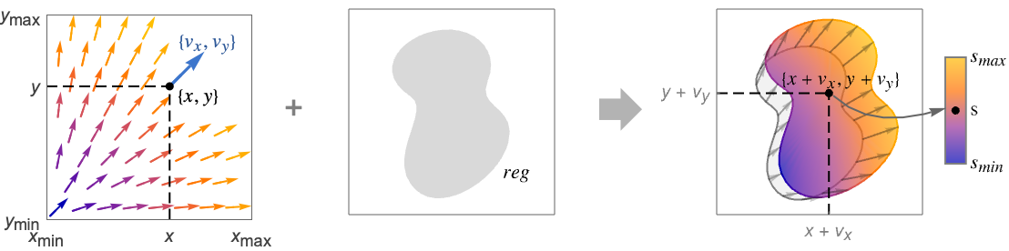
ベクトル場{vx,vy}の変位図プロットを x と y の関数として生成する.
VectorDisplacementPlot[{vx,vy},{x,y}∈reg]
幾何学領域 reg 上に変位図をプロットする.
VectorDisplacementPlot[{{vx,vy},s},…]
スカラー場 s を使って変位図にスタイル付けする.
詳細とオプション
- VectorDisplacementPlotはベクトル場{vx,vy}を使って領域内の点を変位させる.デフォルトで,大小両方の変位が見えるように変位のサイズは自動的にスケールされる.デフォルトで,変位領域は変位の大きさに従って彩色される.
- VectorDisplacementPlotにはGraphicsと同じオプションに以下の追加・変更を加えたものが使える. [全オプションのリスト]
- デフォルトで,変位プロットはもとの領域と変位領域の表現を表示する.
- RegionBoundaryStyleおよびRegionFillingStyleを使ってもとの領域のスタイルを変えることができる.
- 次は,変位矢印を表示するVectorPointsのその他の設定である.
-
Automatic 自動選択された点 "Boundary" reg の境界に沿った点 - デフォルトで,変位矢印はもとの領域内の位置と対応する変位領域内の位置を接続する.
- VectorSizesFullはスケールされた表現ではなく完全な変位を表示する.
全オプションのリスト
例題
すべて開く すべて閉じる例 (5)
指定された変位場について,参照領域と対応する(スケールされた)変形領域をプロットする:
VectorDisplacementPlot[{x, -y}, {x, -1, 1}, {y, -1, 1}]VectorDisplacementPlot[{x, -y}, {x, -1, 1}, {y, -1, 1}, PlotLegends -> Automatic]参照領域内の点から対応する変形領域の点に伸びた変位ベクトルのサンプリングを示す:
VectorDisplacementPlot[{x, -y}, {x, -1, 1}, {y, -1, 1}, VectorPoints -> Automatic]VectorDisplacementPlot[{{x, -y}, x y}, {x, -1, 1}, {y, -1, 1}]底部に沿って固定された横方向に引っ張られているブラケットの変位をプロットする:
VectorDisplacementPlot[IconizedObject[«[image]»], {x, y}∈[image]]VectorDisplacementPlot[{IconizedObject[«[image]»], IconizedObject[«shear stress»]}, {x, y}∈[image]]スコープ (19)
サンプリング (12)
参照領域と変形領域を比較することでスケールされた変位場を可視化する:
VectorDisplacementPlot[{y, x}, {x, -1, 1}, {y, -1, 1}]ベクトルは参照領域内の点から対応する(スケールされた)変形領域内の点まで描かれる:
VectorDisplacementPlot[{y, x}, {x, -1, 1}, {y, -1, 1}, VectorPoints -> Automatic]VectorDisplacementPlot[{y, x} / 2, {x, -1, 1}, {y, -1, 1}, VectorPoints -> "Boundary"]VectorDisplacementPlot[{y, x}, {x, -1, 1}, {y, -1, 1}, VectorPoints -> "Hexagonal"]VectorDisplacementPlot[{y, x} / 2, {x, -1, 1}, {y, -1, 1}, VectorSizes -> Full]VectorDisplacementPlot[{y, x}, {x, -1, 1}, {y, -1, 1}, RegionFunction -> Function[{x, y}, x y ≤ 0.1]]VectorDisplacementPlot[{y, x}, {x, y}∈Disk[]]VectorDisplacementPlot[{y, x}, {x, y}∈HilbertCurve[3, 2]]領域はImplicitRegionでもよい:
ℛ = ImplicitRegion[1 ≤ x^4 + y^4 ≤ 16, {x, y}];VectorDisplacementPlot[{y, x}, {x, y}∈ℛ]領域はParametricRegionでもよい:
ℛ = ParametricRegion[{{s, (1 + t) s ^ 2 - t}, -1 ≤ s ≤ 1 && 0 ≤ t ≤ 1}, {s, t}];VectorDisplacementPlot[{y, x}, {x, y}∈ℛ]領域はMeshRegionでもよい:
ℛ = MeshRegion[Table[(2 + (-1)^t){Cos[π t / 5], Sin[π t / 5]}, {t, 0, 9}], Polygon[{Range[10]}]];VectorDisplacementPlot[{y, x}, {x, y}∈ℛ]領域はBoundaryMeshRegionでもよい:
ℛ = BoundaryMeshRegion[Table[(2 + 0.5(-1)^t){Cos[π t / 8], Sin[π t / 8]}, {t, 0, 16}], Line[{Range[17]}]];VectorDisplacementPlot[{y, x}, {x, y}∈ℛ]プレゼンテーション (7)
変形領域にColorFunctionを指定する:
VectorDisplacementPlot[{x, -y}, {x, y}∈Disk[], ColorFunction -> "Rainbow"]VectorColorFunctionをColorFunctionとは独立で指定する:
VectorDisplacementPlot[{x, -y}, {x, y}∈Disk[], VectorPoints -> Automatic, VectorColorFunction -> "DarkRainbow"]VectorDisplacementPlot[{x, -y}, {x, y}∈Disk[], VectorPoints -> Automatic, VectorColorFunction -> None]VectorDisplacementPlot[{x, -y}, {x, y}∈Disk[], PlotLegends -> Automatic]VectorDisplacementPlot[{{x, -y}, x}, {x, y}∈Disk[], PlotLegends -> Automatic]Meshを含める:
VectorDisplacementPlot[{-y, x}, {x, y}∈Disk[], Mesh -> 5]VectorDisplacementPlot[{-y, x}, {x, y}∈Disk[], Mesh -> 5, VectorSizes -> Full]オプション (64)
AspectRatio (2)
デフォルトで,縦横比はAutomaticである:
VectorDisplacementPlot[{y, x}, {x, -2, 2}, {y, -1, 1}]VectorDisplacementPlot[{y, x}, {x, -2, 2}, {y, -1, 1}, AspectRatio -> 1]BoundaryStyle (3)
デフォルトで,境界スタイルは変形領域の内側の色にマッチする:
VectorDisplacementPlot[{y, x}, {x, -2, 2}, {y, -2, 2}]BoundaryStyleを指定する:
VectorDisplacementPlot[{y, x}, {x, -2, 2}, {y, -2, 2}, BoundaryStyle -> Red]BoundaryStyleはRegionFunctionで切り取られた領域に適用される:
VectorDisplacementPlot[{y, x}, {x, -2, 2}, {y, -2, 2}, BoundaryStyle -> Red, RegionFunction -> Function[{x, y, vx, vy, n}, x^2 + y^2 ≥ 1]]ColorFunction (4)
VectorDisplacementPlot[{1 - x, y}, {x, y}∈Disk[]]VectorDisplacementPlot[{{1 - x, y}, y}, {x, y}∈Disk[]]VectorDisplacementPlot[{1 - x, y}, {x, y}∈Disk[], ColorFunction -> "Rainbow"]カスタムのColorFunctionを使う:
VectorDisplacementPlot[{1 - x, y}, {x, y}∈Disk[], ColorFunction -> Function[{x, y, vx, vy, n}, Hue[vx vy, n, 1]]]ColorFunctionScaling (2)
VectorDisplacementPlot[{1 - x, y}, {x, y}∈Disk[], ColorFunctionScaling -> False]ColorFunctionの個々の引数のスケーリングを制御する:
VectorDisplacementPlot[{1 - x, y}, {x, y}∈Disk[], ColorFunction -> Function[{x, y, vx, vy, n}, Hue[vx vy, n, 1]], ColorFunctionScaling -> {True, True, False, False, True}]Mesh (6)
Meshを指定して変位を可視化する:
VectorDisplacementPlot[{y, x}, {x, 0, 1}, {y, 0, 1}, Mesh -> 5]{VectorDisplacementPlot[{y, x}, {x, 0, 1}, {y, 0, 1}, Mesh -> Full],
VectorDisplacementPlot[{y, x}, {x, 0, 1}, {y, 0, 1}, Mesh -> All]} 方向に10本のメッシュライン,
 方向に5本のメッシュラインを指定する:
VectorDisplacementPlot[{y, x}, {x, 0, 2}, {y, 0, 1}, Mesh -> {10, 5}]VectorDisplacementPlot[{y, x}, {x, 0, 10}, {y, 0, 10}, Mesh -> {{2, 4}, {5, 6, 7}}]VectorDisplacementPlot[{y, x}, {x, 0, 10}, {y, 0, 10}, Mesh -> {{{2, Red}, {4, Blue}}, {5, 6, 7}}]参照領域の境界と塗潰しが削除されると参照領域のメッシュラインも表示されなくなる:
VectorDisplacementPlot[{1, x}, {x, -1, 1}, {y, -1, 1}, Mesh -> 5, RegionBoundaryStyle -> None, RegionFillingStyle -> None]MeshFunctions (2)


MeshStyle (2)
PlotLegends (3)
VectorDisplacementPlot[{x^2 - y^2, x y}, {x, -2, 2}, {y, -2, 2}, PlotLegends -> Automatic]VectorDisplacementPlot[{{x^2 - y^2, x y}, x}, {x, -2, 2}, {y, -2, 2}, PlotLegends -> Automatic]VectorDisplacementPlot[{x^2 - y^2, x y}, {x, -2, 2}, {y, -2, 2}, PlotLegends -> Placed[Automatic, Below]]PlotPoints (1)
PlotRange (3)
デフォルトでPlotRange全体が使われる:
VectorDisplacementPlot[{x^2 - y^2, x y}, {x, -2, 2}, {y, -2, 2}]

VectorDisplacementPlot[{x^2 - y^2, x y}, {x, -2, 2}, {y, -2, 2}, PlotRange -> 3]

VectorDisplacementPlot[{x^2 - y^2, x y}, {x, -2, 2}, {y, -2, 2}, PlotRange -> {{-3, 3}, {-4, 4}}]PlotStyle (4)
VectorDisplacementPlot[{-y, x}, {x, -1, 6}, {y, -2, 3}, PlotStyle -> None]変形領域にTextureを適用する:
VectorDisplacementPlot[{-y, x}, {x, y}∈RegionDifference[Rectangle[{0, 0}, {4, 2}], Disk[{2, 1}, 0.5]], PlotStyle -> Texture[[image]]]PatternFillingを使って変形領域にスタイル付けする:
VectorDisplacementPlot[{-y, x}, {x, y}∈RegionDifference[Rectangle[{0, 0}, {4, 2}], Disk[{2, 1}, 0.5]], PlotStyle -> PatternFilling["Checkerboard"]]ColorFunctionはPlotStyleより優先される:
VectorDisplacementPlot[{-y, x}, {x, y}∈RegionDifference[Rectangle[{0, 0}, {4, 2}], Disk[{2, 1}, 0.5]], ColorFunction -> None, PlotStyle -> Red]RegionBoundaryStyle (2)
RegionFillingStyle (2)
RegionFunction (1)
RegionFunctionを使って参照領域を指定する:
VectorDisplacementPlot[{x^2 - y, y^2 - x}, {x, -3, 3}, {y, -3, 3}, RegionFunction -> Function[{x, y, vx, vy, n}, 1 ≤ x^2 + 2y^2 ≤ 4]]VectorAspectRatio (2)
VectorColorFunction (3)
デフォルトで,VectorColorFunctionがAutomaticならVectorColorFunctionはColorFunctionとマッチする:
VectorDisplacementPlot[{y, -x}, {x, -3, 3}, {y, -3, 3}, VectorPoints -> Automatic, ColorFunction -> GrayLevel]ColorFunctionとは異なるVectorColorFunctionを指定する:
VectorDisplacementPlot[{y, -x}, {x, -3, 3}, {y, -3, 3}, VectorPoints -> Automatic, ColorFunction -> GrayLevel, VectorColorFunction -> "Rainbow"]VectorColorFunctionは使わない:
VectorDisplacementPlot[{y, -x}, {x, -3, 3}, {y, -3, 3}, VectorPoints -> Automatic, VectorColorFunction -> None]VectorColorFunctionScaling (1)
VectorMarkers (3)
デフォルトで,ベクトルは参照領域内の点から対応する変形領域の点まで描かれる:
VectorDisplacementPlot[{y, -x}, {x, -3, 3}, {y, -3, 3}, VectorPoints -> Automatic]VectorDisplacementPlot[{y, -x}, {x, -3, 3}, {y, -3, 3}, VectorPoints -> Automatic, VectorMarkers -> Placed["Arrow", "Center"]]VectorDisplacementPlot[{y, -x}, {x, -3, 3}, {y, -3, 3}, VectorPoints -> Automatic, VectorMarkers -> "Dart"]VectorPoints (9)
VectorDisplacementPlot[{y, -x}, {x, -3, 3}, {y, -3, 3}]VectorDisplacementPlot[{y, -x}, {x, -3, 3}, {y, -3, 3}, VectorPoints -> Automatic]VectorDisplacementPlot[{y, -x}, {x, -3, 3}, {y, -3, 3}, VectorPoints -> "Boundary"]{VectorDisplacementPlot[{y, -x}, {x, -3, 3}, {y, -3, 3}, VectorPoints -> "Fine"], VectorDisplacementPlot[{y, -x}, {x, -3, 3}, {y, -3, 3}, VectorPoints -> "Coarse"]}{VectorDisplacementPlot[{y, -x}, {x, -3, 3}, {y, -3, 3}, VectorPoints -> "Hexagonal"],
VectorDisplacementPlot[{y, -x}, {x, -3, 3}, {y, -3, 3}, VectorPoints -> "Regular"]}

VectorDisplacementPlot[{y, -x}, {x, -3, 3}, {y, -3, 3}, VectorPoints -> 8]

VectorDisplacementPlot[{y, -x}, {x, -3, 3}, {y, -3, 3}, VectorPoints -> {16, 8}]points = {{3, 3}, {-3, 3}, {-3, -3}, {3, -3}};VectorDisplacementPlot[{y, -x}, {x, -3, 3}, {y, -3, 3}, VectorPoints -> points]VectorDisplacementPlot[{y, -x}, {x, y}∈HilbertCurve[3, 2], VectorPoints -> Automatic]VectorRange (2)
VectorDisplacementPlot[{y, x}, {x, -3, 3}, {y, -3, 3}, VectorPoints -> Automatic, VectorRange -> {2, 3}]VectorDisplacementPlot[{y, x}, {x, -3, 3}, {y, -3, 3}, VectorPoints -> Automatic, VectorRange -> {2, 3}, ClippingStyle -> Green]VectorScaling (2)
VectorSizes (4)
デフォルトで,ベクトルは参照領域内の点から変形領域内の対応する点まで描かれる:
VectorDisplacementPlot[(RotationMatrix[π / 4] - IdentityMatrix[2]).{x, y}, {x, -2, 2}, {y, -2, 2}, VectorPoints -> Automatic]VectorDisplacementPlot[(RotationMatrix[π / 4] - IdentityMatrix[2]).{x, y}, {x, -2, 2}, {y, -2, 2}, VectorPoints -> Automatic, VectorSizes -> {0.5, 1}]45°の回転が適切に見えるように変位ベクトルのスケーリングを表示しないようにする:
VectorDisplacementPlot[(RotationMatrix[π / 4] - IdentityMatrix[2]).{x, y}, {x, -2, 2}, {y, -2, 2}, VectorPoints -> "Boundary", VectorSizes -> Full]たとえ変位されたベクトルがなくても,変位ベクトルのスケーリングを表示しないようにする:
VectorDisplacementPlot[(RotationMatrix[π / 4] - IdentityMatrix[2]).{x, y}, {x, -2, 2}, {y, -2, 2}, VectorSizes -> Full]VectorStyle (1)
VectorColorFunctionはVectorStyleよりも優先される:
VectorDisplacementPlot[{x^2 + y^2, x^2 - y^2}, {x, y}∈Disk[], VectorPoints -> "Boundary", VectorColorFunction -> None, VectorStyle -> Red]アプリケーション (23)
基本的なアプリケーション (16)
VectorDisplacementPlot[{2, 1}, {x, 0, 1}, {y, 0, 1}]非常に小さい変位と非常に大きい変位の両方が見えるように,変位は自動的にスケールされる点に注意のこと:
{VectorDisplacementPlot[{0.2, 0.1}, {x, 0, 1}, {y, 0, 1}], VectorDisplacementPlot[{200, 100}, {x, 0, 1}, {y, 0, 1}]}VectorSizesFullを使って変位の実際のサイズを表示する:
VectorDisplacementPlot[{2, 1}, {x, 0, 1}, {y, 0, 1}, VectorSizes -> Full]VectorDisplacementPlot[{2 + x, 1}, {x, 0, 1}, {y, 0, 1}, PlotLegends -> Automatic, VectorSizes -> Full]VectorDisplacementPlot[{{2 + x, 1}, x y}, {x, 0, 1}, {y, 0, 1}, PlotLegends -> Automatic]VectorDisplacementPlot[{2 + x, 1}, {x, 0, 1}, {y, 0, 1}, VectorPoints -> Automatic]
VectorDisplacementPlot[(| | |
| - | - |
| 2 | 0 |
| 0 | 0 |).{x, y}, {x, -1, 1}, {y, -1, 1}, VectorSizes -> Full]
VectorDisplacementPlot[(| | |
| ------ | - |
| -1 / 2 | 0 |
| 0 | 0 |).{x, y}, {x, -1, 1}, {y, -1, 1}, VectorSizes -> Full]

VectorDisplacementPlot[(| | |
| - | ------ |
| 1 | 0 |
| 0 | -1 / 4 |).{x, y}, {x, y}∈Annulus[], VectorSizes -> Full]
VectorDisplacementPlot[(| | |
| - | - |
| 0 | 2 |
| 0 | 0 |).{x, y}, {x, -1, 1}, {y, -1, 1}, VectorSizes -> Full]
VectorDisplacementPlot[(| | |
| - | - |
| 0 | 0 |
| 1 | 0 |).{x, y}, {x, -1, 1}, {y, -1, 1}, VectorSizes -> Full]

VectorDisplacementPlot[(| | |
| - | - |
| 0 | 2 |
| 1 | 0 |).{x, y}, {x, y}∈Annulus[], VectorSizes -> Full]VectorDisplacementPlot[(RotationMatrix[(π/6)] - IdentityMatrix[2]).{x, y}, {x, -1, 1}, {y, -1, 1}, VectorSizes -> Full]VectorDisplacementPlot[((| | |
| - | - |
| 2 | 0 |
| 0 | 1 |).(| | |
| - | - |
| 0 | 2 |
| 1 | 0 |).RotationMatrix[(π/6)] - IdentityMatrix[2]).{x, y}, {x, -1, 1}, {y, -1, 1}, VectorSizes -> Full]VectorDisplacementPlot[Exp[-5(x^2 + y^2)](RotationMatrix[(π/6)] - IdentityMatrix[2]).{x, y}, {x, -1, 1}, {y, -1, 1}, VectorPoints -> Automatic, PlotLegends -> Automatic]VectorDisplacementPlot[Exp[-5(x^2 + y^2)](| | |
| - | - |
| 0 | 2 |
| 1 | 0 |).{x, y}, {x, -1, 1}, {y, -1, 1}, VectorPoints -> Automatic, PlotLegends -> Automatic, Method -> {"ArrowsInFront" -> True}, VectorStyle -> GrayLevel[0.2], VectorColorFunction -> None]固有値と固有ベクトルの可視化 (1)
A = (| | |
| - | -- |
| 4 | -1 |
| 2 | 1 |);その固有値と固有ベクトルを計算する.固有ベクトル  と固有値
と固有値  は固有値問題
 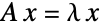 ,
,  を解くが,これは,ここでは,乗算中の行列によって回転されない方向を求めることと解釈できる:
{evals, evecs} = Eigensystem[A]単位円板は の方向には3の倍数分,
 の方向には2の倍数分引き伸ばされる:
VectorDisplacementPlot[(A - IdentityMatrix[2]).{x, y}, {x, y}∈Disk[], PlotLegends -> Automatic, VectorSizes -> Full, Epilog -> Table[Arrow[{{0, 0}, evals[[k]] Normalize[evecs[[k]]]}], {k, 1, Length[evecs]}]]
Area[ImplicitRegion[{x, y}.{x, y} ≤ 1, {x, y}]]{Area@ImplicitRegion[{x, y}.Transpose[Inverse[A]].Inverse[A].{x, y} ≤ 1, {x, y}], π Times@@evals} による乗算が固有ベクトルの方向のものを除くすべてのベクトルを回転させることに注意のこと:
VectorDisplacementPlot[(A - IdentityMatrix[2]).{x, y}, {x, y}∈Disk[], PlotLegends -> Automatic, VectorSizes -> Full, VectorPoints -> "Boundary", Epilog -> Table[Line[{-evals[[k]] Normalize[evecs[[k]]], evals[[k]] Normalize[evecs[[k]]]}], {k, 1, Length[evecs]}]]Aopposite = (| | |
| - | - |
| 2 | 3 |
| 2 | 1 |);
{evals, evecs} = Eigensystem[Aopposite]矢印を使って,負の固有値のために領域が 方向にどのように裏返しになるかを可視化する:
VectorDisplacementPlot[(Aopposite - IdentityMatrix[2]).{x, y}, {x, y}∈Disk[], PlotLegends -> Automatic, VectorSizes -> Full, VectorPoints -> "Boundary", Epilog -> Table[Arrow[{{0, 0}, evals[[k]] Normalize[evecs[[k]]]}], {k, 1, Length[evecs]}]]Azero = (| | |
| - | - |
| 1 | 2 |
| 2 | 4 |);
{evals, evecs} = Eigensystem[Azero]もとの円板が 方向に5の倍数分引き伸ばされるが,
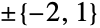 方向には完全に折りたたまれる様子を観察する:
VectorDisplacementPlot[(Azero - IdentityMatrix[2]).{x, y}, {x, y}∈Disk[], VectorSizes -> Full, VectorPoints -> "Boundary"]Arepeated = (| | |
| - | - |
| 2 | 1 |
| 0 | 2 |);
{evals, evecs} = Eigensystem[Arepeated]
VectorDisplacementPlot[(Arepeated - IdentityMatrix[2]).{x, y}, {x, y}∈Disk[], PlotLegends -> Automatic, VectorSizes -> Full, VectorPoints -> "Boundary", Epilog -> Table[Line[{-evals[[k]] Normalize[evecs[[k]]], evals[[k]] Normalize[evecs[[k]]]}], {k, 1, Length[evecs]}]]Arepeated = (| | |
| -- | - |
| 1 | 1 |
| -1 | 1 |);
{evals, evecs} = Eigensystem[Arepeated]固有値の実部のために一様に拡張され,虚部のためにすべてのベクトルが回転される:
VectorDisplacementPlot[(Arepeated - IdentityMatrix[2]).{x, y}, {x, y}∈Disk[], PlotLegends -> Automatic, VectorSizes -> Full, VectorPoints -> "Boundary"]固体力学 (4)
長さ ,高さ
,高さ で両端が大きさ
  のモーメントに従う線形弾性棒について考える:
{h, L} = {1, 4};
Graphics[{LightGray, Rectangle[{-L, -h}, {L, h}], StandardBlue,
	Arrow[Table[{-L - 0.5h Sin[t], 0.5h Cos[t]}, {t, 0, π, 0.1π}]], Arrow[Table[{L + 0.5h Sin[t], 0.5h Cos[t]}, {t, 0, π, 0.1π}]], Text["M", {-L - h, 0}], Text["M", {L + h, 0}]}]
ヤング(Young)率とポアソン(Poisson)比を指定する:
{young, ν} = {30 10^6, 0.25};M = 1;u = (3M/4young h^3){2x y, L^2 - x^2 - ν y^2};VectorDisplacementPlot[u, {x, -L, L}, {y, -h, h}]
σxx = (3M/2h^3)y;
VectorDisplacementPlot[{u, σxx}, {x, -L, L}, {y, -h, h}, PlotLegends -> Automatic]エラスティカは,細く弾性があり伸びることなく曲がる棒である.最初はまっすぐで にある底部が固定され,上端にエラスティカの荷重された端を地面と平行にするのに十分な重さが加えられた垂直エラスティカについて考える.ヤコブ・ベルヌーイ(Jacob Bernoulli)によると弧の長さは以下で与えられる:
S[x_] = Integrate[(1/Sqrt[1 - X^4]), {X, x, 1}, Assumptions -> {0 < x < 1}];S[0.0]同様に,変形されたエラスティカの点の高さは以下で与えられる:
Y[x_] = Integrate[(X^2/Sqrt[1 - X^4]), {X, x, 1}, Assumptions -> {0 < x < 1}];
field = {InverseFunction[S][s], Y[InverseFunction[S][s]]} - {1, s};変形されていないエラスティカのParametricRegionを作成する:
ℛ = ParametricRegion[{1, s}, {{s, 0, S[0]}}];VectorDisplacementPlot[field, {t, s}∈ℛ, VectorSizes -> Full, Epilog -> {Line[{{0, Y[0]}, {0, 0.4}}], Disk[{0, 0.4}, 0.025]}]無限で線形弾性があり原点に半径  の穴があって水平方向に均一な引張荷重がかけられた薄い板について考える:
a = 0.5;
Ω = RegionDifference[Rectangle[{-3, -3}, {3, 3}], Disk[{0, 0}, a]];
VectorPlot[{x, 0}, {x, y}∈Ω, VectorPoints -> Flatten[Table[{x, y}, {x, {-3, 3}}, {y, -3, 3}], 1], VectorMarkers -> "Start", PlotRange -> 4]
{young, ν} = {30 10^6, 0.25};load = 5;平面応力の状態を仮定して,水平および垂直の変位( )と(
)と( )を計算する:
{u, v} = (load a/2young){(2(r/a) + ((a/r))^3(1 + ν) + 2(a/r)(1 + ν)(1 - ((a/r))^2)Cos[2θ] + (a/r)(3 - ν))Cos[θ],
(2ν(r/a) + ((a/r))^3(1 + ν) - 2(a/r)(1 + ν)(1 - ((a/r))^2)Cos[2θ] + (a/r)(1 - 3ν))Sin[θ]} /. {r -> Sqrt[x^2 + y^2], θ -> ArcTan[x, y]};σθθ = (load/2)(1 - (3((a/r))^4 + 1)Cos[2θ] + ((a/r))^2) /. {r -> Sqrt[x^2 + y^2], θ -> ArcTan[x, y]};変形された固体領域をプロットし,無次元フープ応力で彩色する.応力が穴の上下に集中している点に注目のこと:
VectorDisplacementPlot[{{u, v}, (σθθ/load)}, {x, y}∈Ω, PlotLegends -> Automatic, VectorPoints -> Automatic]適用された荷重の大きさにかかわらず,応力の集中係数は3である:
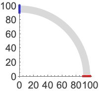
NMaximize[{(σθθ/load), x^2 + y^2 ≥ a^2}, {x, y}]この例では,荷重の増加につれて起こる連続的な変形について考える.
 (赤)で固定され,
  (青)に可変垂直牽引が加えられた細いクォーターアークについて考える:
{r1, r2} = {90, 100};
Ω = DiscretizeRegion[Annulus[{0, 0}, {r1, r2}, {0, (π/2)}]];
平面応力の状態を仮定して変位変数と材料パラメータを定義する:
vars = {{u[x, y], v[x, y]}, {x, y}};
pars = <|"YoungModulus" -> 30 10^6, "PoissonRatio" -> 0.3, "Thickness" -> 0.1, "SolidMechanicsModelForm" -> "PlaneStress"|>;maxLoad = 10000;displacement = NDSolveValue[{SolidMechanicsPDEComponent[vars, pars] == SolidBoundaryLoadValue[x == 0, vars, pars, <|"Pressure" -> {0, -maxLoad}|>], SolidFixedCondition[y == 0, vars, pars]}, {u[x, y], v[x, y]}, {x, y}∈Ω];
shearStrain = SolidMechanicsStrain[vars, pars, displacement][[1, 2]];{minStrain, maxStrain} = Quiet[{NMinimize[shearStrain, {x, y}∈Ω][[1]], NMaximize[shearStrain, {x, y}∈Ω][[1]]}]0から最大値までのすべての荷重に適用される応力について色関数を作成する:
colorfunction = ColorData["Rainbow"][Rescale[#5, {minStrain, maxStrain}]]&;legend = BarLegend[{ColorData["Rainbow"][Rescale[#1, {minStrain, maxStrain}]]&, {minStrain, maxStrain}}, LegendLabel -> "Shear Strain"];一連の荷重値による変形を計算して可視化する.その際,せん断応力を使って変形されたアーチに彩色する:
tb = Table[displacement = NDSolveValue[{SolidMechanicsPDEComponent[vars, pars] == SolidBoundaryLoadValue[x == 0, vars, pars, <|"Pressure" -> {0, -load}|>], SolidFixedCondition[y == 0, vars, pars]}, {u[x, y], v[x, y]}, {x, y}∈Ω];
	shearStrain = SolidMechanicsStrain[vars, pars, displacement][[1, 2]];
	Legended[VectorDisplacementPlot[{displacement, shearStrain}, {x, y}∈Ω, ColorFunction -> colorfunction, ...], legend], {load, 0, maxLoad, maxLoad / 10}];
以下の画像をクリックして荷重を変える.アーチが細いために変位が大きく色は荷重の値すべてに対して一貫している点に注意のこと:
FlipView[tb]複素変数 (1)

f[z_] := (1/z)displacementField = ComplexExpand[ReIm[f[z] - z /. z -> x + I y]]VectorDisplacementPlot[displacementField, {x, y}∈Annulus[{0, 0}, {0.5, 2}], Mesh -> 5, PlotLegends -> Automatic, MeshStyle -> {Black, GrayLevel[0.8]}, VectorSizes -> Full]矢印を使って同心円![TemplateBox[{z}, Abs]=1/2](Files/VectorDisplacementPlot.ja/3.png "TemplateBox[{z}, Abs]=1/2") と
と![TemplateBox[{z}, Abs]=2](Files/VectorDisplacementPlot.ja/4.png "TemplateBox[{z}, Abs]=2") の上の点が
の上の点が  のもとでどのように変換されているかを示す:
VectorDisplacementPlot[displacementField, {x, y}∈Annulus[{0, 0}, {0.5, 2}], VectorSizes -> Full, VectorPoints -> "Boundary", PlotStyle -> None, RegionFillingStyle -> None]地図の投影 (1)
disks = RegionUnion@@Flatten[Table[Disk[{long, lat}, 5], {long, -180, 180, 30}, {lat, -80, 80, 20}]];Show[GeoGraphics[GeoRange -> "World", GeoProjection -> "Equirectangular"], RegionPlot[disks, PlotStyle -> Directive[Gray, Opacity[0.3]], BoundaryStyle -> Gray], AspectRatio -> 1 / 2, ImageSize -> Medium]displacement = {long, (180/π)Log[Abs[Sec[(π/180)lat] + Tan[(π/180)lat]]]} - {long, lat};Show[GeoGraphics[GeoRange -> "World", GeoProjection -> "Mercator"],
VectorDisplacementPlot[displacement, {long, lat}∈disks, PlotPoints -> 50, VectorSizes -> Full, RegionBoundaryStyle -> None, RegionFillingStyle -> None], ImageSize -> Medium]特性と関係 (9)
ListVectorDisplacementPlotを使って変位場データに基づいて変形を可視化する:
data = Table[{{x, y} = RandomReal[{-1, 1}, {2}], {y, x - x ^ 3}}, {300}];ListVectorDisplacementPlot[data, Disk[], VectorPoints -> Automatic]VectorDisplacementPlot3Dを使って変位ベクトル場に関連付けられた3D領域の変形を可視化する:
VectorDisplacementPlot3D[{y, x, -z}, {x, 0, 1}, {y, 0, 1}, {z, 0, 1}, VectorPoints -> "Boundary"]ListVectorDisplacementPlot3Dを使って同じ変形をデータに基づいて可視化する:
data = Table[{{x, y, z} = RandomReal[{0, 1}, {3}], {y, x, -z}}, {300}];ListVectorDisplacementPlot3D[data, Cuboid[], VectorPoints -> "Boundary"]VectorPlotを使ってベクトル場を直接プロットする:
VectorPlot[{-1 - x ^ 2 + y, 1 + x - y ^ 2}, {x, -3, 3}, {y, -3, 3}]StreamPlotでベクトルの代りに流線を使ってプロットする:
StreamPlot[{-1 - x ^ 2 + y, 1 + x - y ^ 2}, {x, -3, 3}, {y, -3, 3}]ListVectorPlotまたはListStreamPlotをデータのプロットに使う:
data = Table[{-1 - x ^ 2 + y, 1 + x - y ^ 2}, {x, -3, 3, 0.2}, {y, -3, 3, 0.2}];{ListVectorPlot[data], ListStreamPlot[data]}VectorDensityPlotを使ってスカラー場の密度プロットを加える:
VectorDensityPlot[{-1 - x ^ 2 + y, 1 + x - y ^ 2}, {x, -3, 3}, {y, -3, 3}]StreamDensityPlotを使ってベクトルの代りに流線をプロットする:
StreamDensityPlot[{-1 - x ^ 2 + y, 1 + x - y ^ 2}, {x, -3, 3}, {y, -3, 3}]ListVectorDensityPlotまたはListStreamDensityPlotをデータのプロットに使う:
data = Table[{{x, y} = RandomReal[{-1.5, 1.5}, {2}], {{y, x - x ^ 3}, Abs[x + y]}}, {300}];{ListVectorDensityPlot[data], ListStreamDensityPlot[data]}LineIntegralConvolutionPlotを使ってベクトル場の線積分のたたみ込みをプロットする:
LineIntegralConvolutionPlot[{-1 - x ^ 2 + y, 1 + x - y ^ 2}, {x, -3, 3}, {y, -3, 3}]VectorPlot3DとStreamPlot3Dを使って3Dベクトル場を可視化する:
{VectorPlot3D[{z, x, x + y}, {x, -1, 1}, {y, -1, 1}, {z, -1, 1}], StreamPlot3D[{z, x, x + y}, {x, -1, 1}, {y, -1, 1}, {z, -1, 1}]}ListVectorPlot3DまたはListStreamPlot3Dを使ってデータでプロットする:
data = Table[{z, x, x + y}, {x, -1, 1}, {y, -1, 1}, {z, -1, 1}];{ListVectorPlot3D[data], ListStreamPlot3D[data]}SliceVectorPlot3Dで曲面上にベクトルをプロットする:
SliceVectorPlot3D[{-y, x, z}, "CenterPlanes", {x, -1, 1}, {y, -1, 1}, {z, -1, 1}]ListSliceVectorPlot3Dを使ってデータでプロットする:
data = Table[{-y, x, z}, {x, -1, 1, 0.1}, {y, -1, 1, 0.1}, {z, -1, 1, 0.1}];ListSliceVectorPlot3D[data, "CenterPlanes"]ComplexVectorPlotまたはComplexStreamPlotを使って複素変数の複素関数をベクトル場としてまたは流線で可視化する:
{ComplexVectorPlot[Sin[3z], {z, 2}], ComplexStreamPlot[Sin[3z], {z, 2}]}GeoVectorPlotを使って地図上にベクトルをプロットする:
GeoVectorPlot[GeoVector[GeoPosition[{{-54.79801473961214, -111.85053058521567},
    {-65.56940402358214, 162.89657500795147}, {-81.67990688759895, -93.36222177594851},
    {7.785750774919734, 95.44840765141487}, {-6.86571958448036, -40.946398330539864},
    { ... 904, "AngularDegrees"]},
   {0.9366099079317551, Quantity[357.70482317743733, "AngularDegrees"]},
   {0.8256817194791912, Quantity[242.07227508889662, "AngularDegrees"]},
{0.2661401145642981, Quantity[152.90003252279325, "AngularDegrees"]}}]]GeoStreamPlotを使ってベクトルの代りに流線をプロットする:
GeoStreamPlot[GeoVector[GeoPosition[{{-54.79801473961214, -111.85053058521567},
    {-65.56940402358214, 162.89657500795147}, {-81.67990688759895, -93.36222177594851},
    {7.785750774919734, 95.44840765141487}, {-6.86571958448036, -40.946398330539864},
    { ... 904, "AngularDegrees"]},
   {0.9366099079317551, Quantity[357.70482317743733, "AngularDegrees"]},
   {0.8256817194791912, Quantity[242.07227508889662, "AngularDegrees"]},
{0.2661401145642981, Quantity[152.90003252279325, "AngularDegrees"]}}]]テキスト
Wolfram Research (2021), VectorDisplacementPlot, Wolfram言語関数, https://reference.wolfram.com/language/ref/VectorDisplacementPlot.html.
CMS
Wolfram Language. 2021. "VectorDisplacementPlot." Wolfram Language & System Documentation Center. Wolfram Research. https://reference.wolfram.com/language/ref/VectorDisplacementPlot.html.
APA
Wolfram Language. (2021). VectorDisplacementPlot. Wolfram Language & System Documentation Center. Retrieved from https://reference.wolfram.com/language/ref/VectorDisplacementPlot.html