


VectorDisplacementPlot
VectorDisplacementPlot[{vx,vy},{x,xmin,xmax},{y,ymin,ymax}]
generates a displacement plot for the vector field {vx,vy} as a function of x and y.
VectorDisplacementPlot[{vx,vy},{x,y}∈reg]
plots the displacement over the geometric region reg.
VectorDisplacementPlot[{{vx,vy},s},…]
uses the scalar field s to style the displacement.
Details and Options
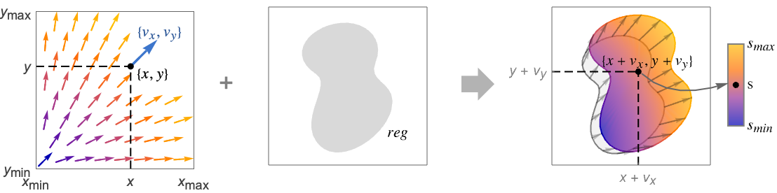
- VectorDisplacementPlot uses the vector field {vx,vy} to displace the points in a region. By default, the size of the displacement is automatically scaled so that both small and large displacements remain visible. The displaced region is by default colored according to the magnitude of the displacement.
- VectorDisplacementPlot has the same options as Graphics, with the following additions and changes: [List of all options]
-
AspectRatio Automatic ratio of height to width BoundaryStyle Automatic how to style the boundary of the displaced region ClippingStyle Automatic how to display arrows outside the vector range ColorFunction Automatic how to color the displaced region ColorFunctionScaling True whether to scale the arguments to ColorFunction EvaluationMonitor None expression to evaluate at every function evaluation Frame True whether to draw a frame around the plot FrameTicks Automatic frame tick marks Mesh None how many mesh lines in each direction to draw MeshFunctions {#1&,#2&} how to determine the placement of mesh lines MeshStyle Automatic the style for mesh lines Method Automatic methods to use for the plot PerformanceGoal $PerformanceGoal aspects of performance to try to optimize PlotLegends None legends to include PlotRange {Full,Full} range of x, y values to include PlotRangePadding Automatic how much to pad the range of values PlotStyle Automatic how to style the deformed region PlotTheme $PlotTheme overall theme for the plot RegionBoundaryStyle Automatic how to style plot region boundaries RegionFillingStyle Automatic how to style plot region interiors RegionFunction (True&) determine what region to include VectorAspectRatio Automatic width to length ratio for arrows VectorColorFunction Automatic how to color arrows VectorColorFunctionScaling True whether to scale the argument to VectorColorFunction VectorMarkers Automatic shape to use for arrows VectorPoints None the number or placement of arrows VectorRange Automatic range of vector lengths to show VectorScaling None how to scale the sizes of arrows VectorSizes Automatic sizes of displayed arrows VectorStyle None how to style arrows WorkingPrecision MachinePrecision precision to use in internal computations - By default, the displacement plot shows a representation of the original region and the displaced region.
- RegionBoundaryStyle and RegionFillingStyle can be used to change the style of the original region.
- Additional settings for VectorPoints to show displacement arrows include:
-
Automatic automatically chosen points "Boundary" points along the boundary of reg - By default, displacement arrows connect locations in the original region with the corresponding displaced locations.
- VectorSizesFull shows the full displacement rather than a scaled representation.
List of all options
Examples
open all close allBasic Examples (5)
Plot a reference region and the corresponding (scaled) deformed region for a specified displacement field:
VectorDisplacementPlot[{x, -y}, {x, -1, 1}, {y, -1, 1}]Include a legend for the norms of the displacements:
VectorDisplacementPlot[{x, -y}, {x, -1, 1}, {y, -1, 1}, PlotLegends -> Automatic]Show a sampling of displacement vectors that extend from points in the reference region to corresponding points in the deformed region:
VectorDisplacementPlot[{x, -y}, {x, -1, 1}, {y, -1, 1}, VectorPoints -> Automatic]Use a scalar field other than the norm of the displacement field to color the deformed region:
VectorDisplacementPlot[{{x, -y}, x y}, {x, -1, 1}, {y, -1, 1}]Plot the displacement for a bracket anchored along the bottom that is being pulled laterally:
VectorDisplacementPlot[IconizedObject[«[image]»], {x, y}∈[image]]Color the displacement according to the shear stress for the bracket:
VectorDisplacementPlot[{IconizedObject[«[image]»], IconizedObject[«shear stress»]}, {x, y}∈[image]]Scope (19)
Sampling (12)
Visualize a scaled displacement field by comparing a reference and a deformed region:
VectorDisplacementPlot[{y, x}, {x, -1, 1}, {y, -1, 1}]Vectors are drawn from points in the reference region to corresponding points in the (scaled) deformed region:
VectorDisplacementPlot[{y, x}, {x, -1, 1}, {y, -1, 1}, VectorPoints -> Automatic]Restrict vectors to points on the boundary:
VectorDisplacementPlot[{y, x} / 2, {x, -1, 1}, {y, -1, 1}, VectorPoints -> "Boundary"]VectorDisplacementPlot[{y, x}, {x, -1, 1}, {y, -1, 1}, VectorPoints -> "Hexagonal"]Displacements can be drawn to scale:
VectorDisplacementPlot[{y, x} / 2, {x, -1, 1}, {y, -1, 1}, VectorSizes -> Full]Use the displacement field over a specified region:
VectorDisplacementPlot[{y, x}, {x, -1, 1}, {y, -1, 1}, RegionFunction -> Function[{x, y}, x y ≤ 0.1]]The domain may be specified by a region:
VectorDisplacementPlot[{y, x}, {x, y}∈Disk[]]VectorDisplacementPlot[{y, x}, {x, y}∈HilbertCurve[3, 2]]The domain may be an ImplicitRegion:
ℛ = ImplicitRegion[1 ≤ x^4 + y^4 ≤ 16, {x, y}];VectorDisplacementPlot[{y, x}, {x, y}∈ℛ]The domain may be a ParametricRegion:
ℛ = ParametricRegion[{{s, (1 + t) s ^ 2 - t}, -1 ≤ s ≤ 1 && 0 ≤ t ≤ 1}, {s, t}];VectorDisplacementPlot[{y, x}, {x, y}∈ℛ]The domain may be a MeshRegion:
ℛ = MeshRegion[Table[(2 + (-1)^t){Cos[π t / 5], Sin[π t / 5]}, {t, 0, 9}], Polygon[{Range[10]}]];VectorDisplacementPlot[{y, x}, {x, y}∈ℛ]The domain may be a BoundaryMeshRegion:
ℛ = BoundaryMeshRegion[Table[(2 + 0.5(-1)^t){Cos[π t / 8], Sin[π t / 8]}, {t, 0, 16}], Line[{Range[17]}]];VectorDisplacementPlot[{y, x}, {x, y}∈ℛ]Presentation (7)
Specify the ColorFunction for the deformed region:
VectorDisplacementPlot[{x, -y}, {x, y}∈Disk[], ColorFunction -> "Rainbow"]Specify the VectorColorFunction independently of the ColorFunction:
VectorDisplacementPlot[{x, -y}, {x, y}∈Disk[], VectorPoints -> Automatic, VectorColorFunction -> "DarkRainbow"]Use a single color for the arrows:
VectorDisplacementPlot[{x, -y}, {x, y}∈Disk[], VectorPoints -> Automatic, VectorColorFunction -> None]Include a legend for the norms of the displacements:
VectorDisplacementPlot[{x, -y}, {x, y}∈Disk[], PlotLegends -> Automatic]Include a legend for the optional scalar field:
VectorDisplacementPlot[{{x, -y}, x}, {x, y}∈Disk[], PlotLegends -> Automatic]Include a Mesh:
VectorDisplacementPlot[{-y, x}, {x, y}∈Disk[], Mesh -> 5]VectorDisplacementPlot[{-y, x}, {x, y}∈Disk[], Mesh -> 5, VectorSizes -> Full]Options (64)
AspectRatio (2)
By default, the aspect ratio is Automatic:
VectorDisplacementPlot[{y, x}, {x, -2, 2}, {y, -1, 1}]VectorDisplacementPlot[{y, x}, {x, -2, 2}, {y, -1, 1}, AspectRatio -> 1]BoundaryStyle (3)
By default, the boundary style matches the interior colors in the deformed region:
VectorDisplacementPlot[{y, x}, {x, -2, 2}, {y, -2, 2}]Specify the BoundaryStyle:
VectorDisplacementPlot[{y, x}, {x, -2, 2}, {y, -2, 2}, BoundaryStyle -> Red]BoundaryStyle applies to regions cut by RegionFunction:
VectorDisplacementPlot[{y, x}, {x, -2, 2}, {y, -2, 2}, BoundaryStyle -> Red, RegionFunction -> Function[{x, y, vx, vy, n}, x^2 + y^2 ≥ 1]]ColorFunction (4)
By default, the deformed region is colored by the norm of the field:
VectorDisplacementPlot[{1 - x, y}, {x, y}∈Disk[]]Specify a scalar field for the colors:
VectorDisplacementPlot[{{1 - x, y}, y}, {x, y}∈Disk[]]VectorDisplacementPlot[{1 - x, y}, {x, y}∈Disk[], ColorFunction -> "Rainbow"]Specify a custom ColorFunction:
VectorDisplacementPlot[{1 - x, y}, {x, y}∈Disk[], ColorFunction -> Function[{x, y, vx, vy, n}, Hue[vx vy, n, 1]]]ColorFunctionScaling (2)
Use the natural range of norm values:
VectorDisplacementPlot[{1 - x, y}, {x, y}∈Disk[], ColorFunctionScaling -> False]Control the scaling of the individual arguments of the ColorFunction:
VectorDisplacementPlot[{1 - x, y}, {x, y}∈Disk[], ColorFunction -> Function[{x, y, vx, vy, n}, Hue[vx vy, n, 1]], ColorFunctionScaling -> {True, True, False, False, True}]Mesh (6)
Specify a Mesh to visualize the displacements:
VectorDisplacementPlot[{y, x}, {x, 0, 1}, {y, 0, 1}, Mesh -> 5]Show the initial and final sampling mesh:
{VectorDisplacementPlot[{y, x}, {x, 0, 1}, {y, 0, 1}, Mesh -> Full],
	VectorDisplacementPlot[{y, x}, {x, 0, 1}, {y, 0, 1}, Mesh -> All]}
Specify 10 mesh lines in the ![]() direction and 5 in the
direction and 5 in the ![]() direction:
direction:
VectorDisplacementPlot[{y, x}, {x, 0, 2}, {y, 0, 1}, Mesh -> {10, 5}]Use mesh lines at specific values:
VectorDisplacementPlot[{y, x}, {x, 0, 10}, {y, 0, 10}, Mesh -> {{2, 4}, {5, 6, 7}}]Highlight specific mesh lines:
VectorDisplacementPlot[{y, x}, {x, 0, 10}, {y, 0, 10}, Mesh -> {{{2, Red}, {4, Blue}}, {5, 6, 7}}]Mesh lines are suppressed in the reference region if the boundary and filling of the reference region are removed:
VectorDisplacementPlot[{1, x}, {x, -1, 1}, {y, -1, 1}, Mesh -> 5, RegionBoundaryStyle -> None, RegionFillingStyle -> None]MeshFunctions (2)
By default, the mesh lines are in the ![]() and
and ![]() directions:
directions:
VectorDisplacementPlot[{Sin[y], Cos[x]}, {x, y}∈Disk[{0, 0}, 3], Mesh -> 6]Use circular and radial mesh lines:
VectorDisplacementPlot[{Sin[y], Cos[x]}, {x, y}∈Disk[{0, 0}, 3], Mesh -> 6, MeshFunctions -> {#1^2 + #2^2&, ArcTan[#1, #2]&}]MeshStyle (2)
PlotLegends (3)
Include a legend to show the color range of vector norms:
VectorDisplacementPlot[{x^2 - y^2, x y}, {x, -2, 2}, {y, -2, 2}, PlotLegends -> Automatic]Include a legend for the optional scalar field:
VectorDisplacementPlot[{{x^2 - y^2, x y}, x}, {x, -2, 2}, {y, -2, 2}, PlotLegends -> Automatic]Control the placement of the legend:
VectorDisplacementPlot[{x^2 - y^2, x y}, {x, -2, 2}, {y, -2, 2}, PlotLegends -> Placed[Automatic, Below]]PlotPoints (1)
PlotRange (3)
The full PlotRange is used by default:
VectorDisplacementPlot[{x^2 - y^2, x y}, {x, -2, 2}, {y, -2, 2}]Specify an explicit limit that is shared by the ![]() and
and ![]() directions:
directions:
VectorDisplacementPlot[{x^2 - y^2, x y}, {x, -2, 2}, {y, -2, 2}, PlotRange -> 3]Specify different plot ranges in the ![]() and
and ![]() directions:
directions:
VectorDisplacementPlot[{x^2 - y^2, x y}, {x, -2, 2}, {y, -2, 2}, PlotRange -> {{-3, 3}, {-4, 4}}]PlotStyle (4)
Remove the filling for the deformed region:
VectorDisplacementPlot[{-y, x}, {x, -1, 6}, {y, -2, 3}, PlotStyle -> None]Apply a Texture to the deformed region:
VectorDisplacementPlot[{-y, x}, {x, y}∈RegionDifference[Rectangle[{0, 0}, {4, 2}], Disk[{2, 1}, 0.5]], PlotStyle -> Texture[[image]]]Use PatternFilling to style the deformed region:
VectorDisplacementPlot[{-y, x}, {x, y}∈RegionDifference[Rectangle[{0, 0}, {4, 2}], Disk[{2, 1}, 0.5]], PlotStyle -> PatternFilling["Checkerboard"]]ColorFunction has precedence over PlotStyle:
VectorDisplacementPlot[{-y, x}, {x, y}∈RegionDifference[Rectangle[{0, 0}, {4, 2}], Disk[{2, 1}, 0.5]], ColorFunction -> None, PlotStyle -> Red]RegionBoundaryStyle (2)
Specify the boundary color of the reference region:
VectorDisplacementPlot[{x y, x}, {x, y}∈Annulus[], RegionBoundaryStyle -> Red]Remove the boundary of the reference region:
VectorDisplacementPlot[{x y, x}, {x, y}∈Annulus[], RegionBoundaryStyle -> None]RegionFillingStyle (2)
RegionFunction (1)
Use a RegionFunction to specify the reference region:
VectorDisplacementPlot[{x^2 - y, y^2 - x}, {x, -3, 3}, {y, -3, 3}, RegionFunction -> Function[{x, y, vx, vy, n}, 1 ≤ x^2 + 2y^2 ≤ 4]]VectorAspectRatio (2)
The default aspect ratio for a vector marker is 1/4:
VectorDisplacementPlot[{y, -x}, {x, -3, 3}, {y, -3, 3}, VectorPoints -> Automatic]Specify the relative width of a vector marker:
VectorDisplacementPlot[{y, -x}, {x, -3, 3}, {y, -3, 3}, VectorPoints -> Automatic, VectorAspectRatio -> 1 / 2]VectorColorFunction (3)
By default, if VectorColorFunction is Automatic, then the VectorColorFunction matches the ColorFunction:
VectorDisplacementPlot[{y, -x}, {x, -3, 3}, {y, -3, 3}, VectorPoints -> Automatic, ColorFunction -> GrayLevel]Specify a VectorColorFunction that is different from the ColorFunction:
VectorDisplacementPlot[{y, -x}, {x, -3, 3}, {y, -3, 3}, VectorPoints -> Automatic, ColorFunction -> GrayLevel, VectorColorFunction -> "Rainbow"]Use no VectorColorFunction:
VectorDisplacementPlot[{y, -x}, {x, -3, 3}, {y, -3, 3}, VectorPoints -> Automatic, VectorColorFunction -> None]VectorColorFunctionScaling (1)
VectorMarkers (3)
By default, vectors are drawn from points in the reference region to corresponding points in the deformed region:
VectorDisplacementPlot[{y, -x}, {x, -3, 3}, {y, -3, 3}, VectorPoints -> Automatic]Center the markers at the sampled points:
VectorDisplacementPlot[{y, -x}, {x, -3, 3}, {y, -3, 3}, VectorPoints -> Automatic, VectorMarkers -> Placed["Arrow", "Center"]]Use a named appearance to draw the vectors:
VectorDisplacementPlot[{y, -x}, {x, -3, 3}, {y, -3, 3}, VectorPoints -> Automatic, VectorMarkers -> "Dart"]VectorPoints (9)
No vectors are shown by default:
VectorDisplacementPlot[{y, -x}, {x, -3, 3}, {y, -3, 3}]Show vectors sampled from the entire original region:
VectorDisplacementPlot[{y, -x}, {x, -3, 3}, {y, -3, 3}, VectorPoints -> Automatic]Sample vectors from the boundary of the region:
VectorDisplacementPlot[{y, -x}, {x, -3, 3}, {y, -3, 3}, VectorPoints -> "Boundary"]Use symbolic names to specify the density of vectors:
{VectorDisplacementPlot[{y, -x}, {x, -3, 3}, {y, -3, 3}, VectorPoints -> "Fine"], VectorDisplacementPlot[{y, -x}, {x, -3, 3}, {y, -3, 3}, VectorPoints -> "Coarse"]}Use symbolic names to specify the arrangement of vectors:
{VectorDisplacementPlot[{y, -x}, {x, -3, 3}, {y, -3, 3}, VectorPoints -> "Hexagonal"],
	VectorDisplacementPlot[{y, -x}, {x, -3, 3}, {y, -3, 3}, VectorPoints -> "Regular"]}
Specify the number of vectors in the ![]() and
and ![]() directions:
directions:
VectorDisplacementPlot[{y, -x}, {x, -3, 3}, {y, -3, 3}, VectorPoints -> 8]Specify a different number of vectors in the ![]() and
and ![]() directions:
directions:
VectorDisplacementPlot[{y, -x}, {x, -3, 3}, {y, -3, 3}, VectorPoints -> {16, 8}]Give specific locations for vectors:
points = {{3, 3}, {-3, 3}, {-3, -3}, {3, -3}};VectorDisplacementPlot[{y, -x}, {x, -3, 3}, {y, -3, 3}, VectorPoints -> points]Along a curve, vectors are equally spaced by default:
VectorDisplacementPlot[{y, -x}, {x, y}∈HilbertCurve[3, 2], VectorPoints -> Automatic]VectorRange (2)
Specify the range of vector norms:
VectorDisplacementPlot[{y, x}, {x, -3, 3}, {y, -3, 3}, VectorPoints -> Automatic, VectorRange -> {2, 3}]VectorDisplacementPlot[{y, x}, {x, -3, 3}, {y, -3, 3}, VectorPoints -> Automatic, VectorRange -> {2, 3}, ClippingStyle -> Green]VectorScaling (2)
By default, vectors extend from points in the reference region to corresponding points in the deformed region:
VectorDisplacementPlot[{Sin[y], Cos[x]}, {x, y}∈Annulus[], VectorPoints -> Automatic]Set all vectors to have the same size:
VectorDisplacementPlot[{Sin[y], Cos[x]}, {x, y}∈Annulus[], VectorPoints -> Automatic, VectorScaling -> None]VectorSizes (4)
By default, vectors extend from points in the reference region to corresponding points in the deformed region:
VectorDisplacementPlot[(RotationMatrix[π / 4] - IdentityMatrix[2]).{x, y}, {x, -2, 2}, {y, -2, 2}, VectorPoints -> Automatic]Specify the range of arrow lengths:
VectorDisplacementPlot[(RotationMatrix[π / 4] - IdentityMatrix[2]).{x, y}, {x, -2, 2}, {y, -2, 2}, VectorPoints -> Automatic, VectorSizes -> {0.5, 1}]Suppress scaling of the displacement vectors so that a rotation of 45° looks appropriate:
VectorDisplacementPlot[(RotationMatrix[π / 4] - IdentityMatrix[2]).{x, y}, {x, -2, 2}, {y, -2, 2}, VectorPoints -> "Boundary", VectorSizes -> Full]Suppress scaling of the displacement vectors even if no vectors are displayed:
VectorDisplacementPlot[(RotationMatrix[π / 4] - IdentityMatrix[2]).{x, y}, {x, -2, 2}, {y, -2, 2}, VectorSizes -> Full]VectorStyle (1)
VectorColorFunction has precedence over VectorStyle:
VectorDisplacementPlot[{x^2 + y^2, x^2 - y^2}, {x, y}∈Disk[], VectorPoints -> "Boundary", VectorColorFunction -> None, VectorStyle -> Red]Applications (23)
Basic Applications (16)
A constant displacement field moves each point in the reference region by the same amount:
VectorDisplacementPlot[{2, 1}, {x, 0, 1}, {y, 0, 1}]Note that the displacements are automatically scaled so that very small and very large displacements are both visible:
{VectorDisplacementPlot[{0.2, 0.1}, {x, 0, 1}, {y, 0, 1}], VectorDisplacementPlot[{200, 100}, {x, 0, 1}, {y, 0, 1}]}Use VectorSizesFull to display the actual sizes of displacements:
VectorDisplacementPlot[{2, 1}, {x, 0, 1}, {y, 0, 1}, VectorSizes -> Full]Color is used to indicate the magnitude of the displacements:
VectorDisplacementPlot[{2 + x, 1}, {x, 0, 1}, {y, 0, 1}, PlotLegends -> Automatic, VectorSizes -> Full]Color the region by a different scalar function:
VectorDisplacementPlot[{{2 + x, 1}, x y}, {x, 0, 1}, {y, 0, 1}, PlotLegends -> Automatic]Use arrows to indicate initial and final locations for a sample points:
VectorDisplacementPlot[{2 + x, 1}, {x, 0, 1}, {y, 0, 1}, VectorPoints -> Automatic]Visualize a dilation in the ![]() direction:
direction:
VectorDisplacementPlot[(| | |
| - | - |
| 2 | 0 |
| 0 | 0 |).{x, y}, {x, -1, 1}, {y, -1, 1}, VectorSizes -> Full]Visualize a contraction in the ![]() direction:
direction:
VectorDisplacementPlot[(| | |
| ------ | - |
| -1 / 2 | 0 |
| 0 | 0 |).{x, y}, {x, -1, 1}, {y, -1, 1}, VectorSizes -> Full]Visualize a dilation in the ![]() direction and a contraction in the
direction and a contraction in the ![]() direction:
direction:
VectorDisplacementPlot[(| | |
| - | ------ |
| 1 | 0 |
| 0 | -1 / 4 |).{x, y}, {x, y}∈Annulus[], VectorSizes -> Full]Visualize a shear in the ![]() direction:
direction:
VectorDisplacementPlot[(| | |
| - | - |
| 0 | 2 |
| 0 | 0 |).{x, y}, {x, -1, 1}, {y, -1, 1}, VectorSizes -> Full]Visualize a shear in the ![]() direction:
direction:
VectorDisplacementPlot[(| | |
| - | - |
| 0 | 0 |
| 1 | 0 |).{x, y}, {x, -1, 1}, {y, -1, 1}, VectorSizes -> Full]Visualize a combined shear in the ![]() and
and ![]() directions:
directions:
VectorDisplacementPlot[(| | |
| - | - |
| 0 | 2 |
| 1 | 0 |).{x, y}, {x, y}∈Annulus[], VectorSizes -> Full]Visualize a rotation about the origin:
VectorDisplacementPlot[(RotationMatrix[(π/6)] - IdentityMatrix[2]).{x, y}, {x, -1, 1}, {y, -1, 1}, VectorSizes -> Full]Combine a rotation, a shear and a dilation:
VectorDisplacementPlot[((| | |
| - | - |
| 2 | 0 |
| 0 | 1 |).(| | |
| - | - |
| 0 | 2 |
| 1 | 0 |).RotationMatrix[(π/6)] - IdentityMatrix[2]).{x, y}, {x, -1, 1}, {y, -1, 1}, VectorSizes -> Full]Visualize a rotation for points near the origin:
VectorDisplacementPlot[Exp[-5(x^2 + y^2)](RotationMatrix[(π/6)] - IdentityMatrix[2]).{x, y}, {x, -1, 1}, {y, -1, 1}, VectorPoints -> Automatic, PlotLegends -> Automatic]Visualize a shear for points near the origin:
VectorDisplacementPlot[Exp[-5(x^2 + y^2)](| | |
| - | - |
| 0 | 2 |
| 1 | 0 |).{x, y}, {x, -1, 1}, {y, -1, 1}, VectorPoints -> Automatic, PlotLegends -> Automatic, Method -> {"ArrowsInFront" -> True}, VectorStyle -> GrayLevel[0.2], VectorColorFunction -> None]Visualizing Eigenvalues and Eigenvectors (1)
A = (| | |
| - | -- |
| 4 | -1 |
| 2 | 1 |);Compute its eigenvalues and eigenvectors. Eigenvectors ![]() and eigenvalues
and eigenvalues ![]() solve the eigenvalue problem
solve the eigenvalue problem ![]() ,
, ![]() , which can be interpreted here as finding directions that are not rotated by the matrix under multiplication:
, which can be interpreted here as finding directions that are not rotated by the matrix under multiplication:
{evals, evecs} = Eigensystem[A]The unit disk is stretched by a factor of 3 in the ![]() direction and a factor of 2 in the
direction and a factor of 2 in the ![]() direction:
direction:
VectorDisplacementPlot[(A - IdentityMatrix[2]).{x, y}, {x, y}∈Disk[], PlotLegends -> Automatic, VectorSizes -> Full, Epilog -> Table[Arrow[{{0, 0}, evals[[k]] Normalize[evecs[[k]]]}], {k, 1, Length[evecs]}]]Area[ImplicitRegion[{x, y}.{x, y} ≤ 1, {x, y}]]The area of the interior of the resulting ellipse is the product of the eigenvalues times the original area:
{Area@ImplicitRegion[{x, y}.Transpose[Inverse[A]].Inverse[A].{x, y} ≤ 1, {x, y}], π Times@@evals}Note that multiplication by ![]() rotates all vectors except those in the eigenvector directions:
rotates all vectors except those in the eigenvector directions:
VectorDisplacementPlot[(A - IdentityMatrix[2]).{x, y}, {x, y}∈Disk[], PlotLegends -> Automatic, VectorSizes -> Full, VectorPoints -> "Boundary", Epilog -> Table[Line[{-evals[[k]] Normalize[evecs[[k]]], evals[[k]] Normalize[evecs[[k]]]}], {k, 1, Length[evecs]}]]Define a matrix with one positive and one negative eigenvalue:
Aopposite = (| | |
| - | - |
| 2 | 3 |
| 2 | 1 |);
{evals, evecs} = Eigensystem[Aopposite]Use arrows to visualize how the region turns inside out in the ![]() direction because of the negative eigenvalue:
direction because of the negative eigenvalue:
VectorDisplacementPlot[(Aopposite - IdentityMatrix[2]).{x, y}, {x, y}∈Disk[], PlotLegends -> Automatic, VectorSizes -> Full, VectorPoints -> "Boundary", Epilog -> Table[Arrow[{{0, 0}, evals[[k]] Normalize[evecs[[k]]]}], {k, 1, Length[evecs]}]]Define a matrix with a zero eigenvalue:
Azero = (| | |
| - | - |
| 1 | 2 |
| 2 | 4 |);
{evals, evecs} = Eigensystem[Azero]Observe that the original disk is stretched by a factor of 5 in the ![]() direction, but completely collapsed in the
direction, but completely collapsed in the ![]() direction:
direction:
VectorDisplacementPlot[(Azero - IdentityMatrix[2]).{x, y}, {x, y}∈Disk[], VectorSizes -> Full, VectorPoints -> "Boundary"]Define a matrix with a repeated real eigenvalue:
Arepeated = (| | |
| - | - |
| 2 | 1 |
| 0 | 2 |);
{evals, evecs} = Eigensystem[Arepeated]Observe that the vectors are rotated unless they point in the ![]() direction:
direction:
VectorDisplacementPlot[(Arepeated - IdentityMatrix[2]).{x, y}, {x, y}∈Disk[], PlotLegends -> Automatic, VectorSizes -> Full, VectorPoints -> "Boundary", Epilog -> Table[Line[{-evals[[k]] Normalize[evecs[[k]]], evals[[k]] Normalize[evecs[[k]]]}], {k, 1, Length[evecs]}]]Define a matrix with complex eigenvalues:
Arepeated = (| | |
| -- | - |
| 1 | 1 |
| -1 | 1 |);
{evals, evecs} = Eigensystem[Arepeated]The real part of the eigenvalues causes a uniform dilation and the imaginary part causes every vector to rotate:
VectorDisplacementPlot[(Arepeated - IdentityMatrix[2]).{x, y}, {x, y}∈Disk[], PlotLegends -> Automatic, VectorSizes -> Full, VectorPoints -> "Boundary"]Solid Mechanics (4)
Consider a linearly elastic bar of length ![]() and height
and height ![]() subjected to a moment of magnitude
subjected to a moment of magnitude ![]() at both ends:
at both ends:
{h, L} = {1, 4};
Graphics[{LightGray, Rectangle[{-L, -h}, {L, h}], StandardBlue,
	Arrow[Table[{-L - 0.5h Sin[t], 0.5h Cos[t]}, {t, 0, π, 0.1π}]], Arrow[Table[{L + 0.5h Sin[t], 0.5h Cos[t]}, {t, 0, π, 0.1π}]], Text["M", {-L - h, 0}], Text["M", {L + h, 0}]}]
Specify Young's modulus and Poisson's ratio:
{young, ν} = {30 10^6, 0.25};Specify the magnitude of the applied moment:
M = 1;The resulting displacement vector is:
u = (3M/4young h^3){2x y, L^2 - x^2 - ν y^2};VectorDisplacementPlot[u, {x, -L, L}, {y, -h, h}]The only nontrivial stress is the normal stress in the ![]() direction:
direction:
σxx = (3M/2h^3)y;VectorDisplacementPlot[{u, σxx}, {x, -L, L}, {y, -h, h}, PlotLegends -> Automatic]An elastica is a thin, elastic rod that bends without stretching. Consider an initially straight, vertical elastica that is clamped at the bottom end at ![]() and loaded with a weight at the top end that is sufficiently large to make the elastica parallel to the ground at the loaded end. Jacob Bernoulli famously found that the arc length is given by:
and loaded with a weight at the top end that is sufficiently large to make the elastica parallel to the ground at the loaded end. Jacob Bernoulli famously found that the arc length is given by:
S[x_] = Integrate[(1/Sqrt[1 - X^4]), {X, x, 1}, Assumptions -> {0 < x < 1}];The total length of the elastica is:
S[0.0]Similarly, the height of a point on the deformed elastica is given by:
Y[x_] = Integrate[(X^2/Sqrt[1 - X^4]), {X, x, 1}, Assumptions -> {0 < x < 1}];In terms of the parameter ![]() , the resulting displacement field is:
, the resulting displacement field is:
field = {InverseFunction[S][s], Y[InverseFunction[S][s]]} - {1, s};Create a ParametricRegion for the undeformed elastica:
ℛ = ParametricRegion[{1, s}, {{s, 0, S[0]}}];Visualize the deformed elastica with the weight attached:
VectorDisplacementPlot[field, {t, s}∈ℛ, VectorSizes -> Full, Epilog -> {Line[{{0, Y[0]}, {0, 0.4}}], Disk[{0, 0.4}, 0.025]}]Consider an infinite, linearly elastic, thin plate with a hole of radius ![]() at the origin with a uniform tensile load in the horizontal direction:
at the origin with a uniform tensile load in the horizontal direction:
a = 0.5;
Ω = RegionDifference[Rectangle[{-3, -3}, {3, 3}], Disk[{0, 0}, a]];
VectorPlot[{x, 0}, {x, y}∈Ω, VectorPoints -> Flatten[Table[{x, y}, {x, {-3, 3}}, {y, -3, 3}], 1], VectorMarkers -> "Start", PlotRange -> 4]
Specify Young's modulus and Poisson's ratio ![]() :
:
{young, ν} = {30 10^6, 0.25};Specify the magnitude of the applied tensile load:
load = 5;Compute the horizontal (![]() ) and vertical (
) and vertical (![]() ) displacements assuming a state of plane stress:
) displacements assuming a state of plane stress:
{u, v} = (load a/2young){(2(r/a) + ((a/r))^3(1 + ν) + 2(a/r)(1 + ν)(1 - ((a/r))^2)Cos[2θ] + (a/r)(3 - ν))Cos[θ],
(2ν(r/a) + ((a/r))^3(1 + ν) - 2(a/r)(1 + ν)(1 - ((a/r))^2)Cos[2θ] + (a/r)(1 - 3ν))Sin[θ]} /. {r -> Sqrt[x^2 + y^2], θ -> ArcTan[x, y]};σθθ = (load/2)(1 - (3((a/r))^4 + 1)Cos[2θ] + ((a/r))^2) /. {r -> Sqrt[x^2 + y^2], θ -> ArcTan[x, y]};Plot the deformed solid region and color it by the dimensionless hoop stress. Note the stress concentration at the top and bottom of the hole:
VectorDisplacementPlot[{{u, v}, (σθθ/load)}, {x, y}∈Ω, PlotLegends -> Automatic, VectorPoints -> Automatic]The stress concentration factor is 3, regardless of the magnitude of the applied load:
NMaximize[{(σθθ/load), x^2 + y^2 ≥ a^2}, {x, y}]This example considers a sequence of deformations that correspond to an increasing load.
Consider a thin quarter-arch that is fixed at ![]() (red) with a variable vertical traction applied at
(red) with a variable vertical traction applied at ![]() (blue):
(blue):
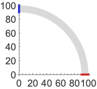
{r1, r2} = {90, 100};
Ω = DiscretizeRegion[Annulus[{0, 0}, {r1, r2}, {0, (π/2)}]];
Assume a state of plane stress and define the displacement variables and the material parameters:
vars = {{u[x, y], v[x, y]}, {x, y}};
pars = <|"YoungModulus" -> 30 10^6, "PoissonRatio" -> 0.3, "Thickness" -> 0.1, "SolidMechanicsModelForm" -> "PlaneStress"|>;maxLoad = 10000;Compute the displacement and shear strain for the maximum load:
displacement = NDSolveValue[{SolidMechanicsPDEComponent[vars, pars] == SolidBoundaryLoadValue[x == 0, vars, pars, <|"Pressure" -> {0, -maxLoad}|>], SolidFixedCondition[y == 0, vars, pars]}, {u[x, y], v[x, y]}, {x, y}∈Ω];
shearStrain = SolidMechanicsStrain[vars, pars, displacement][[1, 2]];
Compute the minimum and maximum values of the shear strain:
{minStrain, maxStrain} = Quiet[{NMinimize[shearStrain, {x, y}∈Ω][[1]], NMaximize[shearStrain, {x, y}∈Ω][[1]]}]Create a color function for the strains that applies for all load values from zero load up to the maximum:
colorfunction = ColorData["Rainbow"][Rescale[#5, {minStrain, maxStrain}]]&;Create a legend that applies for all load values:
legend = BarLegend[{ColorData["Rainbow"][Rescale[#1, {minStrain, maxStrain}]]&, {minStrain, maxStrain}}, LegendLabel -> "Shear Strain"];Compute and visualize the deformations for a sequence of load values, using the shear strain to color the deformed arch:
tb = Table[displacement = NDSolveValue[{SolidMechanicsPDEComponent[vars, pars] == SolidBoundaryLoadValue[x == 0, vars, pars, <|"Pressure" -> {0, -load}|>], SolidFixedCondition[y == 0, vars, pars]}, {u[x, y], v[x, y]}, {x, y}∈Ω];
	shearStrain = SolidMechanicsStrain[vars, pars, displacement][[1, 2]];
	Legended[VectorDisplacementPlot[{displacement, shearStrain}, {x, y}∈Ω, ColorFunction -> colorfunction, ...], legend], {load, 0, maxLoad, maxLoad / 10}];
Click the following image to cycle through the loads. Note that the displacements are large because the arch is thin and that the colors are consistent across all of the load values:
FlipView[tb]Complex Variables (1)
f[z_] := (1/z)Compute the displacement field:
displacementField = ComplexExpand[ReIm[f[z] - z /. z -> x + I y]]Visualize the complex transformation and note that lines are mapped to circles:
VectorDisplacementPlot[displacementField, {x, y}∈Annulus[{0, 0}, {0.5, 2}], Mesh -> 5, PlotLegends -> Automatic, MeshStyle -> {Black, GrayLevel[0.8]}, VectorSizes -> Full]Use arrows to illustrate how points on the concentric circles ![]() and
and ![]() are transformed under
are transformed under ![]() :
:
VectorDisplacementPlot[displacementField, {x, y}∈Annulus[{0, 0}, {0.5, 2}], VectorSizes -> Full, VectorPoints -> "Boundary", PlotStyle -> None, RegionFillingStyle -> None]Map Projections (1)
Generate a number of disks and form their union:
disks = RegionUnion@@Flatten[Table[Disk[{long, lat}, 5], {long, -180, 180, 30}, {lat, -80, 80, 20}]];Superimpose the disks on a map of the world with an equirectangular projection:
Show[GeoGraphics[GeoRange -> "World", GeoProjection -> "Equirectangular"], RegionPlot[disks, PlotStyle -> Directive[Gray, Opacity[0.3]], BoundaryStyle -> Gray], AspectRatio -> 1 / 2, ImageSize -> Medium]Specify the displacement from the equirectangular projection to a Mercator projection:
displacement = {long, (180/π)Log[Abs[Sec[(π/180)lat] + Tan[(π/180)lat]]]} - {long, lat};Show the deformed disks on a map with the Mercator projection:
Show[GeoGraphics[GeoRange -> "World", GeoProjection -> "Mercator"],
	VectorDisplacementPlot[displacement, {long, lat}∈disks, PlotPoints -> 50, VectorSizes -> Full, RegionBoundaryStyle -> None, RegionFillingStyle -> None], ImageSize -> Medium]
Properties & Relations (9)
Use ListVectorDisplacementPlot to visualize a deformation based on displacement field data:
data = Table[{{x, y} = RandomReal[{-1, 1}, {2}], {y, x - x ^ 3}}, {300}];ListVectorDisplacementPlot[data, Disk[], VectorPoints -> Automatic]Use VectorDisplacementPlot3D to visualize the deformation of a 3D region associated with a displacement vector field:
VectorDisplacementPlot3D[{y, x, -z}, {x, 0, 1}, {y, 0, 1}, {z, 0, 1}, VectorPoints -> "Boundary"]Use ListVectorDisplacementPlot3D to visualize the same deformation based on data:
data = Table[{{x, y, z} = RandomReal[{0, 1}, {3}], {y, x, -z}}, {300}];ListVectorDisplacementPlot3D[data, Cuboid[], VectorPoints -> "Boundary"]Use VectorPlot to directly plot a vector field:
VectorPlot[{-1 - x ^ 2 + y, 1 + x - y ^ 2}, {x, -3, 3}, {y, -3, 3}]Use StreamPlot to plot with streamlines instead of vectors:
StreamPlot[{-1 - x ^ 2 + y, 1 + x - y ^ 2}, {x, -3, 3}, {y, -3, 3}]Use ListVectorPlot or ListStreamPlot for plotting data:
data = Table[{-1 - x ^ 2 + y, 1 + x - y ^ 2}, {x, -3, 3, 0.2}, {y, -3, 3, 0.2}];{ListVectorPlot[data], ListStreamPlot[data]}Use VectorDensityPlot to add a density plot of the scalar field:
VectorDensityPlot[{-1 - x ^ 2 + y, 1 + x - y ^ 2}, {x, -3, 3}, {y, -3, 3}]Use StreamDensityPlot to plot streamlines instead of vectors:
StreamDensityPlot[{-1 - x ^ 2 + y, 1 + x - y ^ 2}, {x, -3, 3}, {y, -3, 3}]Use ListVectorDensityPlot or ListStreamDensityPlot for plotting data:
data = Table[{{x, y} = RandomReal[{-1.5, 1.5}, {2}], {{y, x - x ^ 3}, Abs[x + y]}}, {300}];{ListVectorDensityPlot[data], ListStreamDensityPlot[data]}Use LineIntegralConvolutionPlot to plot the line integral convolution of a vector field:
LineIntegralConvolutionPlot[{-1 - x ^ 2 + y, 1 + x - y ^ 2}, {x, -3, 3}, {y, -3, 3}]Use VectorPlot3D and StreamPlot3D to visualize 3D vector fields:
{VectorPlot3D[{z, x, x + y}, {x, -1, 1}, {y, -1, 1}, {z, -1, 1}], StreamPlot3D[{z, x, x + y}, {x, -1, 1}, {y, -1, 1}, {z, -1, 1}]}Use ListVectorPlot3D or ListStreamPlot3D to plot with data:
data = Table[{z, x, x + y}, {x, -1, 1}, {y, -1, 1}, {z, -1, 1}];{ListVectorPlot3D[data], ListStreamPlot3D[data]}Plot vectors on surfaces with SliceVectorPlot3D:
SliceVectorPlot3D[{-y, x, z}, "CenterPlanes", {x, -1, 1}, {y, -1, 1}, {z, -1, 1}]Use ListSliceVectorPlot3D to plot with data:
data = Table[{-y, x, z}, {x, -1, 1, 0.1}, {y, -1, 1, 0.1}, {z, -1, 1, 0.1}];ListSliceVectorPlot3D[data, "CenterPlanes"]Use ComplexVectorPlot or ComplexStreamPlot to visualize a complex function of a complex variable as a vector field or with streamlines:
{ComplexVectorPlot[Sin[3z], {z, 2}], ComplexStreamPlot[Sin[3z], {z, 2}]}Use GeoVectorPlot to plot vectors on a map:
GeoVectorPlot[GeoVector[GeoPosition[{{-54.79801473961214, -111.85053058521567},
    {-65.56940402358214, 162.89657500795147}, {-81.67990688759895, -93.36222177594851},
    {7.785750774919734, 95.44840765141487}, {-6.86571958448036, -40.946398330539864},
    { ... 904, "AngularDegrees"]},
   {0.9366099079317551, Quantity[357.70482317743733, "AngularDegrees"]},
   {0.8256817194791912, Quantity[242.07227508889662, "AngularDegrees"]},
   {0.2661401145642981, Quantity[152.90003252279325, "AngularDegrees"]}}]]
Use GeoStreamPlot to plot streamlines instead of vectors:
GeoStreamPlot[GeoVector[GeoPosition[{{-54.79801473961214, -111.85053058521567},
    {-65.56940402358214, 162.89657500795147}, {-81.67990688759895, -93.36222177594851},
    {7.785750774919734, 95.44840765141487}, {-6.86571958448036, -40.946398330539864},
    { ... 904, "AngularDegrees"]},
   {0.9366099079317551, Quantity[357.70482317743733, "AngularDegrees"]},
   {0.8256817194791912, Quantity[242.07227508889662, "AngularDegrees"]},
{0.2661401145642981, Quantity[152.90003252279325, "AngularDegrees"]}}]]Text
Wolfram Research (2021), VectorDisplacementPlot, Wolfram Language function, https://reference.wolfram.com/language/ref/VectorDisplacementPlot.html.
CMS
Wolfram Language. 2021. "VectorDisplacementPlot." Wolfram Language & System Documentation Center. Wolfram Research. https://reference.wolfram.com/language/ref/VectorDisplacementPlot.html.
APA
Wolfram Language. (2021). VectorDisplacementPlot. Wolfram Language & System Documentation Center. Retrieved from https://reference.wolfram.com/language/ref/VectorDisplacementPlot.html